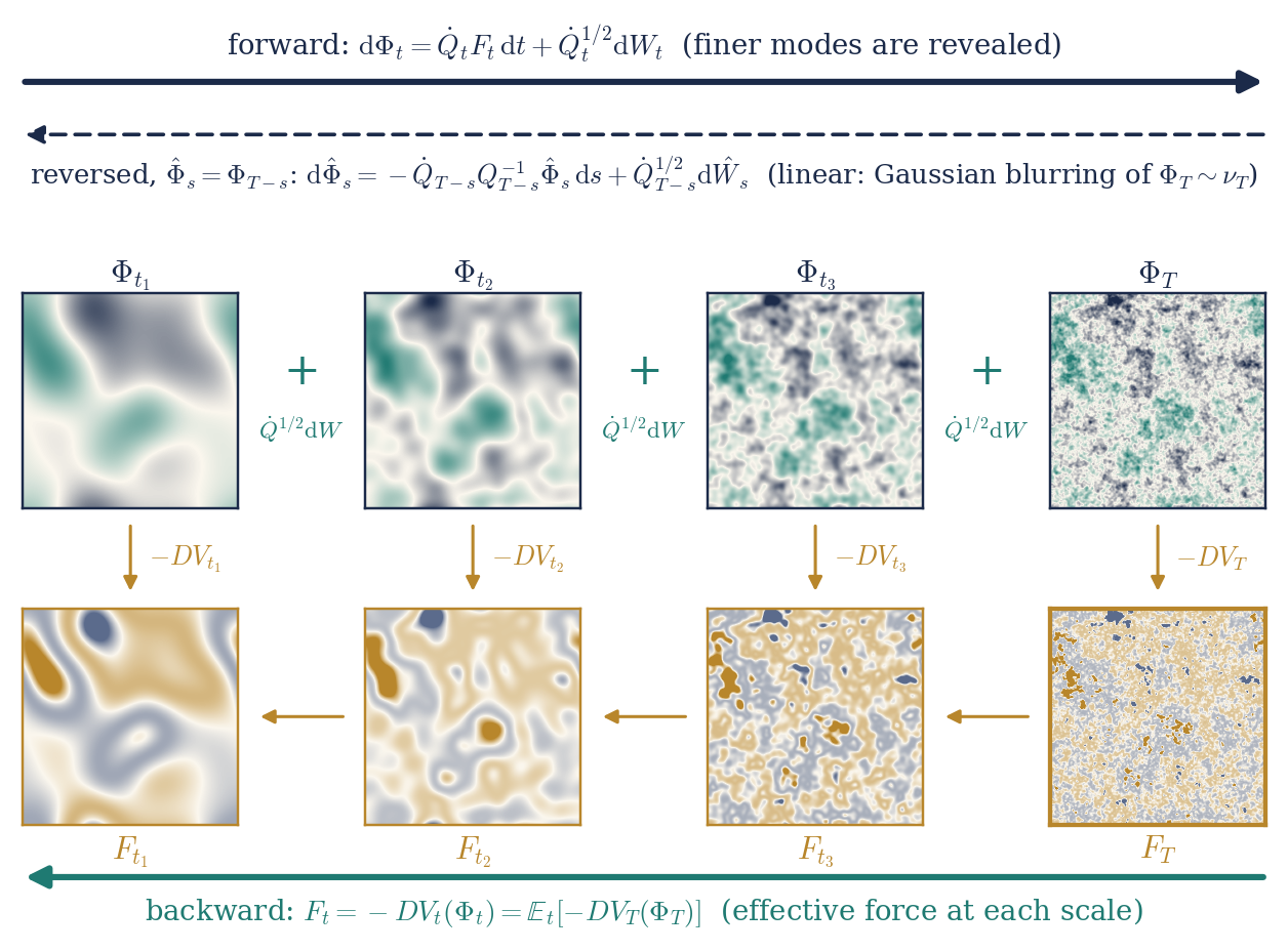
Vertical: \(F_t = -
\mathrm{D} V_t (\Phi_t)\). Dashed: backward the process is
linear (Gaussian blurring). Force to first order,
\(- (\lambda / 3) H_3 (\Phi_t ; c_t)\).
A Constructive Introduction to Quantum Field Theory
Forward–backward equations
Massimiliano Gubinelli | University of Oxford
Joint work with Sarah-Jean Meyer, with the use of AI
SISSA lectures, Lecture 4 — notes: Lecture 4,
§§7–8
So far. Stochastic quantisation of the GFF; the field at resolution \(t\) is a martingale of smooth fields; observables are martingales in the filtration of finite-resolution measurements.
Today. Interactions, still indexed by the resolution \(t \in [0, T]\).
Generate the measure three ways: renormalisation, optimal control, filtering.
They meet in one system for a field and a force: the force coordinates.
Potentials: the value function generates them; Legendre; Wetterich.
Next time (Lecture 5): observables, and the field equation with its sub-Gaussian noise.
Caveat. Statements marked
Fix \(V_T\) and \(\nu_T \propto \mathrm{e}^{- V_T} \mu^{Q_T}\). Let \(S_t = Q_T - Q_t\), the covariance still unresolved at resolution \(t\).
Renormalisation. Split the covariance into shells and integrate them out. At every resolution the field is again a Gibbs measure, driven by an effective force.
Optimal control. Steer the Gaussian field by a drift, at the least cost. The effective potential is the value function, and the Polchinski equation is the dynamic programming equation.
Filtering. The field at resolution \(t\) is a noisy observation of the terminal field. The conditional law is the posterior, the force is what the observation reveals, and backward in resolution its dynamics is linear and Gaussian, started from \(\nu_T\).
They produce the same process.
Three ways to generate the interacting measure
Lecture 4
Finite volume \(\mathbb{T}^d_L\), terminal resolution \(T < \infty\) (UV cutoff), interaction \(V_T\) bounded below, e.g.
Definition.
The interaction felt at resolution \(t\) once the scales \([t, T]\) are integrated out; \(V_0 (0) = - \log Z_T\) is the free energy.
Proposition.
At every resolution the field is again a Gibbs measure: reference \(Q_t\), potential \(V_t\).
The measure-valued martingale \(t \mapsto \mu_t^{X_t}\) goes from \(\nu_T\) (\(t = 0\)) to \(\delta_{X_T}\) (\(t = T\)): a stochastic localisation of \(\nu_T\) (Eldan), adapted to the covariance profile.
Proof of the marginals. Under \(\mathbb{P}_0\), \(X_T = X_t + (X_T - X_t)\) with independent increment \(\sim \mu^{Q_{T, t}}\), so
Theorem.
The effective force \(F\) is a \(\mathbb{P}\)-martingale: an observable field of the interacting theory.
Proof. Density process \(M_t = Z_T^{- 1} \mathrm{e}^{- V_t (X_t)}\). It is a martingale, so by Itô it has no drift, \(\mathrm{d} M_t = - M_t \langle \mathrm{D} V_t (X_t), \dot{Q}_t^{1 / 2} \mathrm{d} W_t \rangle\). Girsanov: \(W^{\mathbb{P}}_t = W_t + \int_0^t \dot{Q}_s^{1 / 2} \mathrm{D} V_s (X_s) \hspace{0.17em} \mathrm{d} s\). Finally \(\mathrm{D} V_t (\phi) = \mu_t^{\phi} (\mathrm{D} V_T)\).
Under \(\mathbb{P}_0\), \(X\) is the GFF martingale, with generator \(L_t = \frac{1}{2} \text{Tr} (\dot{Q}_t \mathrm{D}^2)\). The function
is space-time harmonic: this is the Polchinski equation. Since \(\mathrm{d} \mathbb{P}/ \mathrm{d} \mathbb{P}_0 |_{\mathcal{F}_t} = h_t (X_t)\),
Simplest case: a Brownian motion conditioned on its endpoint, \(h_t =\) Gaussian density of the remaining increment, and the drift of the bridge.
The Polchinski process is the Doob \(h\)-transform of the GFF martingale by \(\mathrm{e}^{- V_T}\): the free field conditioned to end with the law \(\nu_T\).
Read as an equation for an unknown pair \((\Phi, F)\):
The field is driven forward by a force determined backward from the terminal field.
No Polchinski equation needed; \(\nu_T = \text{Law} (\Phi_T)\) from the solution.
Strategy: solve with renormalised \(V_T\), estimates uniform in \(T\) and volume, take limits.
\(\Phi\) is not an observable (a semimartingale); observables are built from the noise and from \(F\).
Vertical: \(F_t = -
\mathrm{D} V_t (\Phi_t)\). Dashed: backward the process is
linear (Gaussian blurring). Force to first order,
\(- (\lambda / 3) H_3 (\Phi_t ; c_t)\).
Theorem.
Proof. \(u_t = \mathrm{e}^{- V_t} = \mathrm{e}^{\frac{1}{2} \Delta_{Q_{T, t}}} u_T\), \(\Delta_Q = \text{Tr} (Q \mathrm{D}^2)\), solves the backward heat equation \(\partial_t u_t = - \frac{1}{2} \text{Tr} (\dot{Q}_t \mathrm{D}^2 u_t)\). Insert \(\mathrm{D}^2 u = (\mathrm{D} V \otimes \mathrm{D} V - \mathrm{D}^2 V) u\).
Nonlinear term: generates new, nonlocal interactions (trees). |
Trace term: contracts pairs of fields with the shell covariance \(\dot{Q}_t \hspace{0.17em} \mathrm{d} t\): loops. |
A backward Hamilton–Jacobi equation; \(h \propto \mathrm{e}^{- V}\) is a Cole–Hopf transform.
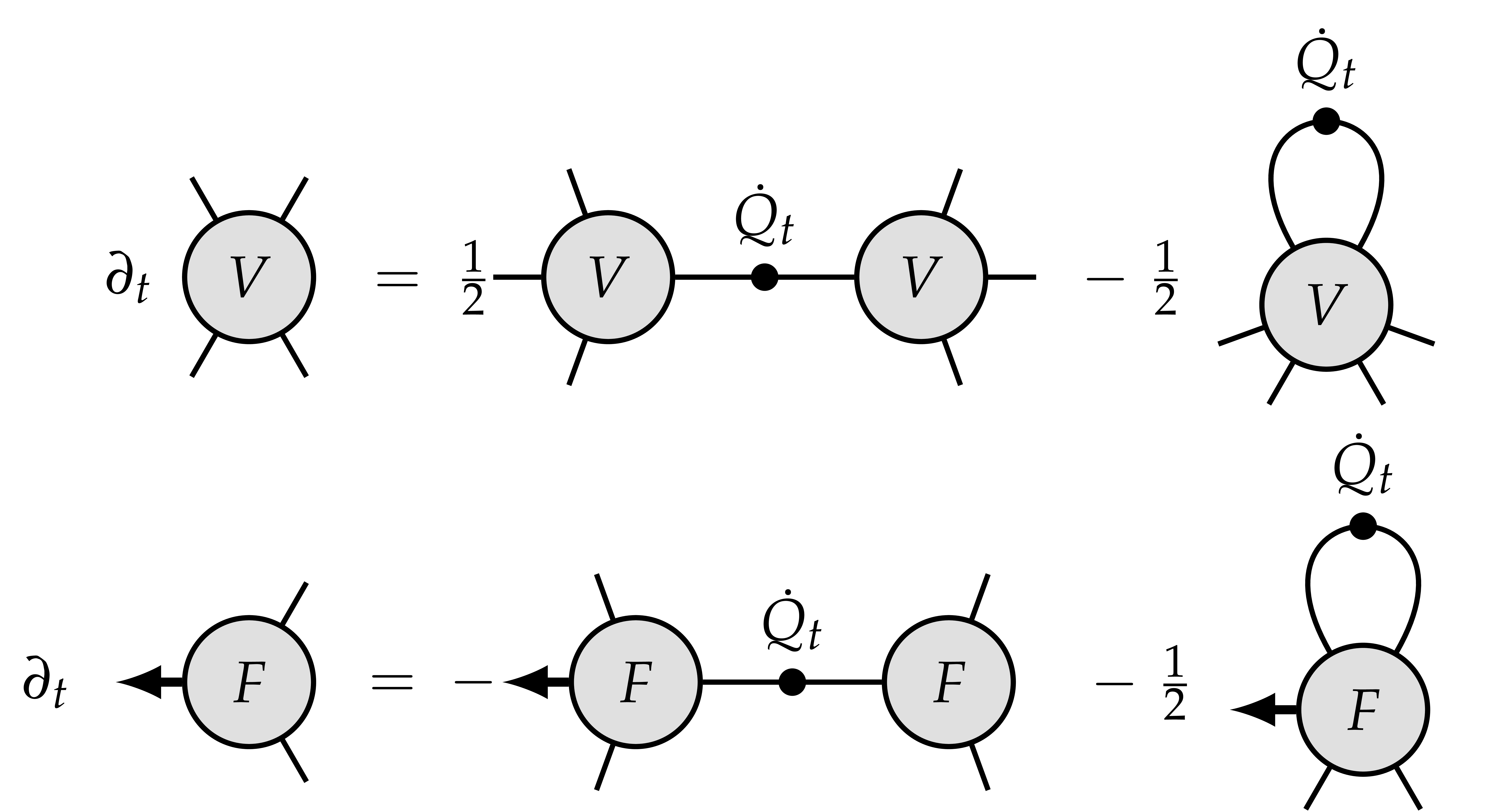
Blob: derivatives of \(V_t\) or of the force. Dotted line: \(\dot{Q}_t\). Tree term and loop term; iterating gives the connected Feynman graphs.
\(\mathbb{H}_a\): adapted drifts with \(\mathbb{E} \int_0^T \|u_s \|^2 < \infty\); \(X^u = X + \int_0^{\cdot} \dot{Q}_s^{1 / 2} u_s \hspace{0.17em} \mathrm{d} s\).
Theorem.
Optimal feedback \(u^{\ast}_s = - \dot{Q}_s^{1 / 2} \mathrm{D} V_s (X^{u^{\ast}}_s)\), \(\text{Law} (X^{u^{\ast}}_T) = \nu_T\). \(V_t\) is the value function; Polchinski is the HJB equation.
Proof (verification). Itô \(+\) Polchinski:
Euler–Lagrange. Perturb \(u \to u + \varepsilon v\):
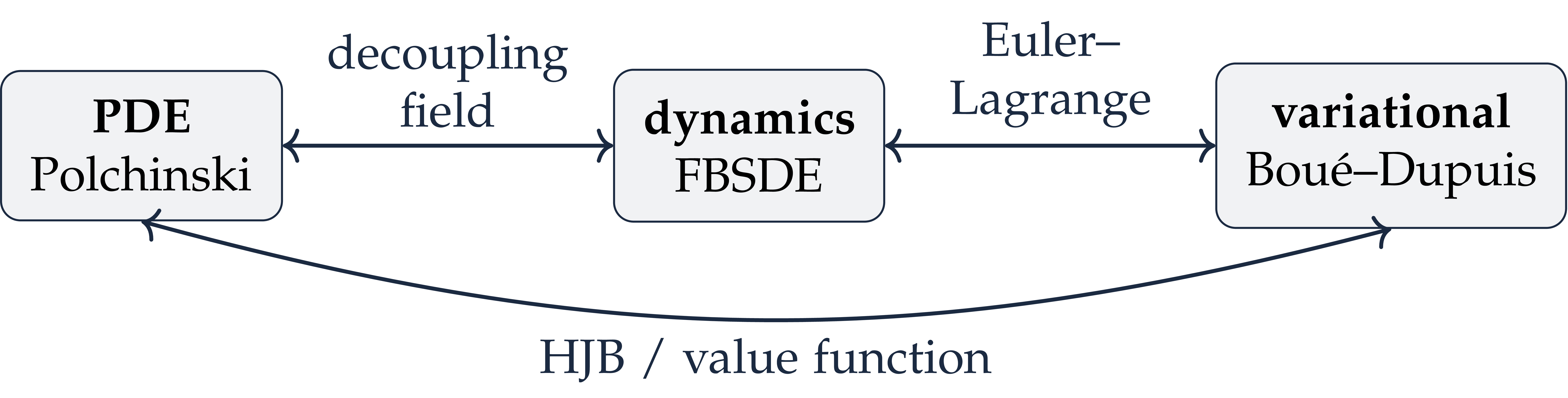
Entropy. \(\frac{1}{2} \mathbb{E}_0 \int \|u\|^2 \geqslant \text{Ent} (\text{Law} (X^u) | \text{Law} (X))\): a pathwise lift of the Gibbs principle
Useful because adapted drifts can be built scale by scale, as functionals of \(X\).
Generating functional:
Bounds uniform in \(T\) \(\Rightarrow\) tightness, moments, identification of limits.
\(\Phi^4_3\). The leading drift \(u_s \approx - \frac{\lambda}{3} \dot{Q}_s^{1 / 2} : X_s^3\): has divergent cost,
Change variables \(u = - \frac{\lambda}{3} \dot{Q}^{1 / 2} : X^3 : + r\), then paracontrolled changes of variables: the singular terms become explicit polynomials in Wick powers of \(X\), cancelled by the counterterms, and the remainder is coercive. Uniform control in Besov/paracontrolled norms \(=\) construction of \(\Phi^4_3\). Barashkov–Gubinelli, Duke 2020; EJP 2021
Minimise
subject to \(\dot{x} = b (x, u)\), \(x_t = x\). Hamiltonian:
Theorem.
State forward, costate backward: a two-point boundary problem.
The costate is the Lagrange multiplier of the constraint \(\dot{x} = b\); an optimal control is a critical point of the Hamiltonian.
Next: why this holds, and what \(p\) is.
Pontryagin–Boltyanskii–Gamkrelidze–Mishchenko 1962.
First variation. Perturb \(u \to u + \varepsilon v\); the state varies by \(\xi = \partial_{\varepsilon} x\),
The costate equation \(\dot{p} = - \partial_x \mathcal{H}\) is exactly what makes
Integrating, with \(p_T = - Dg (x_T)\):
HJB. Dynamic programming over \([t, t + \mathrm{d} t]\):
Hamilton's equations for \(\mathcal{H}_{\ast}\) are its characteristics, and along them \(p_s = - \mathrm{D} V (s, x_s)\): the costate is the force the future exerts on the present.
State \(=\) field, \(b = \dot{Q}_s^{1 / 2} u\), \(\ell = \frac{1}{2} \|u\|^2\), \(g = V_T\). \(\mathcal{H}\) is maximised at \(u = \dot{Q}_s^{1 / 2} p\):
a free particle with mass matrix \(\dot{Q}_s^{- 1}\), and no dependence on the state \(x\).
Without noise: \(\dot{p} = 0\), \(\dot{x} = \dot{Q} p\): the shear \(\Sigma_t : (x, p) \mapsto (x + S_t p, p)\), with \(S_t := Q_T - Q_t\) the covariance still unresolved. All interaction is in \(p = - \mathrm{D} V_T (x + S_T p)\): trees. HJB \(=\) Polchinski without the trace.
With noise (Bismut 1973, Peng 1990): the costate solves a BSDE
with \(\Upsilon \mathrm{d} W\) the price of adaptedness. Here \(\partial_x \mathcal{H}= 0\): the costate is a martingale, \(p_t = - \mathrm{D} V_t (X_t) = F_t\).
The Itô term turns HJB into Polchinski: quadratic part \(=\) trees, trace term \(=\) loops.
The FBSDE is the stochastic Hamiltonian system: field \(=\) state, force \(=\) costate.
Here \(\dot{S}_t = - \dot{Q}_t\), \(S_T = 0\). Optimal control \(u_t = \dot{Q}_t^{1 / 2} p_t\), with costate \(p_t = F_t\):
\(F_t (\cdot)\) is the decoupling field, \(F_t = F_t (\Phi_t)\); Burgers is its quasilinear PDE, and \(\Upsilon\) the martingale representation integrand of the costate.
In Burgers: transport term \(- \mathrm{D} F [\dot{Q} F]\) \(\leftarrow\) drift of the state; Itô term \(- \frac{1}{2} \text{Tr} (\dot{Q} \mathrm{D}^2 F)\) \(\leftarrow\) noise.
The shear \(\Sigma_t\) is the flow of the transport part: its characteristics.
All covariance operators are functions of \(A\); \(K = Q_T^{- 1}\), \(J_t = KQ_t\). Since \(\mathrm{d} \mathbb{P}/ \mathrm{d} \mathbb{P}_0\) depends on \(X_T\) only, given \(\Phi_T\) the interacting field is the Gaussian bridge:
with \(\zeta\), \(B\) independent of \(\Phi_T\). Signal \(\Phi_T\), with prior \(\nu_T\); observation \((\Phi_s)_{s \leqslant t}\), pulled towards the hidden field.
Proposition.
Posterior: \(\mu_t^{\Phi_t} (\mathrm{d} y) \propto \mathrm{e}^{\langle S_t^{- 1} \Phi_t, y \rangle - \frac{1}{2} \langle y, \mathcal{R}_t y \rangle} \nu_T (\mathrm{d} y)\), \(\mathcal{R}_t = S_t^{- 1} - Q_T^{- 1}\) the precision gained: the regulator.
\(F_t =\mathbb{E}_t [S_t^{- 1} (\Phi_T - \Phi_t)]\): \(\dot{Q}_t F_t\) is the posterior mean of the pull, \(\psi_t = \Phi_t + S_t F_t\), and \(W\) is the innovation. The Polchinski SDE is the observation equation in its own filtration.
Filter equation: \(\mathrm{d} \mathbb{E}_t [G (\Phi_T)] = \langle \text{Cov}_t (G, \Phi_T), S_t^{- 1} \dot{Q}_t^{1 / 2} \mathrm{d} W_t \rangle\).
Reverse the resolution, \(\hat{\Phi}_s = \Phi_{T - s}\):
\(\mathrm{d} \mathbb{P}/ \mathrm{d} \mathbb{P}_0\) depends only on the starting point \(X_T\): the transition kernels are those of the Gaussian reference, only the initial law changes. A linear process with Gaussian transitions, not a Gaussian process.
Backward: blur the interacting field with Gaussian noise, \(\Phi_t = J_t \Phi_T + \zeta_t\); this does not know the interaction. Forward: Polchinski undoes the blurring, all the interaction is in the drift.
Time reversal (\(t > 0\), finite cutoff): forward drift \(b_t = \dot{Q}_t F_t\), backward drift \(\beta_t = - \dot{Q}_t Q_t^{- 1} x\), and \(b_t + \beta_t = \dot{Q}_t \mathrm{D} \log p_t\): reversal compensates the drift up to the score of the density at that scale (Nelson's osmotic velocity). So \(F\) is the score of \(\nu_t\) relative to \(\mu^{Q_t}\), \(\psi_t\) is the denoiser (Tweedie), and the noise is \(\omega_t = - J_t \mathrm{D} \log p_t (\Phi_t)\).
The Polchinski process is a denoising diffusion whose data distribution is the interacting measure.
In the stochastic localisation literature the observation is written as a linear measurement: with \(j_t = S_t^{- 1} \Phi_t\),
signal-to-noise ratio \(\mathcal{R}_t\). The posterior is an exponential family in \(j\), with log-partition function \(\mathcal{K}_t (j) = \text{log} \int \mathrm{e}^{\langle j, y \rangle - \frac{1}{2} \langle y, \mathcal{R}_t y \rangle} \nu_T (\mathrm{d} y)\):
\(\psi_t = \mathrm{D} \mathcal{K}_t (j_t)\), \(\text{Cov}_t = \mathrm{D}^2 \mathcal{K}_t (j_t)\), \(\mathrm{d} j_t = \dot{\mathcal{R}}_t \psi_t \hspace{0.17em} \mathrm{d} t + \dot{\mathcal{R}}_t^{1 / 2} \hspace{0.17em} \mathrm{d} W_t\);
\(\partial_t \mathcal{K}+ \frac{1}{2} \text{Tr} (\dot{\mathcal{R}} \mathrm{D}^2 \mathcal{K}) + \frac{1}{2} \langle \mathrm{D} \mathcal{K}, \dot{\mathcal{R}} \mathrm{D} \mathcal{K} \rangle = 0\): Polchinski in the variable \(j\).
Eldan's basic scheme is the profile with \(\mathcal{R}_t = t\), \(N\) a Brownian motion, run to \(t = \infty\): the profile of Lectures 6–7.
Eldan 2013; El Alaoui–Montanari 2022; Bauerschmidt–Bodineau–Dagallier 2024
|
Renormalisation |
Control |
Filtering |
\(\Phi_t\) |
field at resolution \(t\) |
state |
observation; posterior mean, Gaussian prior |
\(F_t\) |
effective force |
costate |
posterior mean of the terminal force |
\(W\) |
fresh fluctuation of the shell |
noise of the controlled field |
innovation |
\(S_t\) |
unresolved covariance |
free motion from \(t\) to \(T\) |
posterior covariance, Gaussian prior |
\(\psi_t = \Phi_t + S_t F_t\) |
mean of the conditional law |
terminal state, free prediction |
posterior mean |
\(\text{Cov}_t\) |
covariance of the conditional law |
\(S_t - S_t \mathrm{D}^2 V_t S_t\) |
posterior covariance |
\(V_t\) |
effective potential |
value function |
\(-\)log-likelihood ratio of the observation, up to \(\log Z_T\) |
\(\psi_t - \Phi_t = S_t F_t\): the force is what the interaction adds to the estimate, in units of the free propagator \(S_t\), and \(\text{Cov}_t\) replaces \(S_t\) as the propagator.
At finite \(T\) the force is a closed observable, \(F_t =\mathbb{E}_t [F_T]\), and for \(\Phi^4\) it is local:
As \(T \to \infty\)
\(F\) should converge as an observable. In \(d = 2\) it is closed, \(F_{\infty} = - \frac{\lambda}{3} : \Phi_{\infty}^3\):. In \(d = 3\) a closed limit \(F_t =\mathbb{E}_t F_{\infty}\) would let the DS identity pass to \(t \to \infty\), and conditioning on \(\sigma (\Phi_{\infty})\) would give an integrable logarithmic derivative of \(\Phi^4_3\) as a function of the field: not expected (Albeverio–Liang–Zegarlinski 2006: the regularised ones do not converge in \(L^2\)). Locality of the limiting force is the crux of the construction.
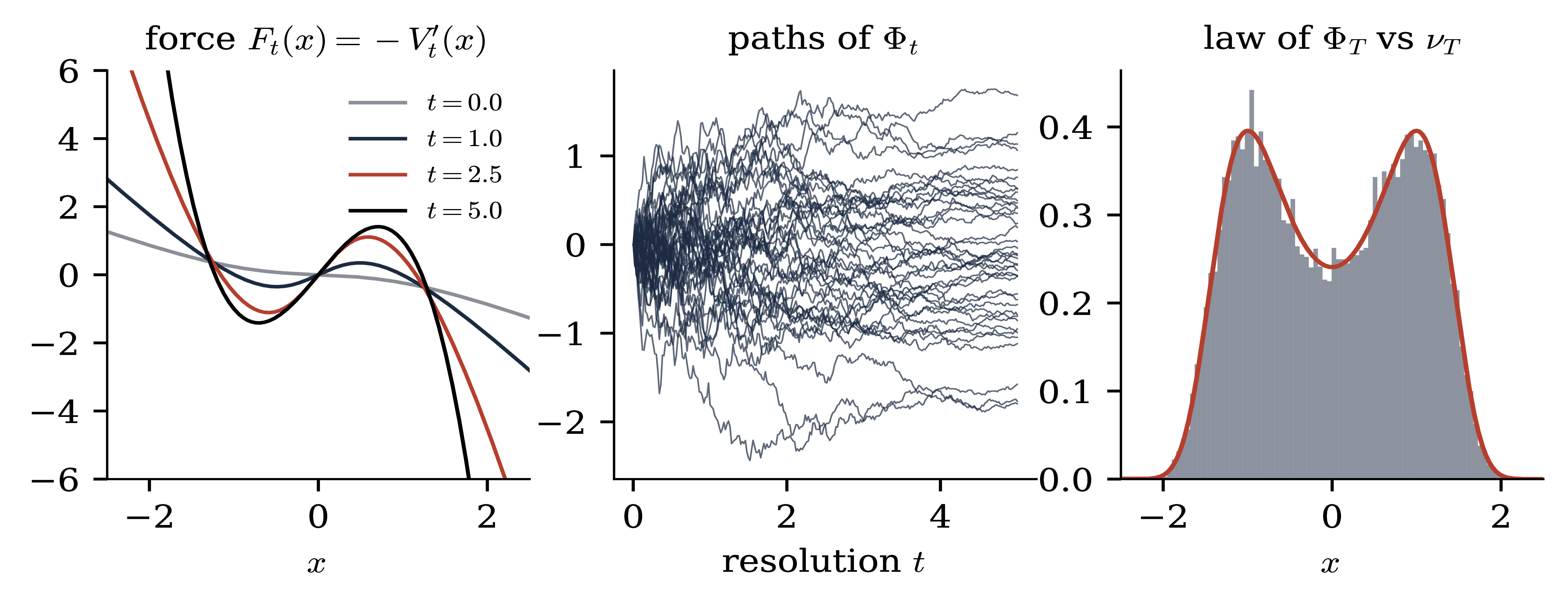
\(Q_t = 1 - \mathrm{e}^{-
t}\), \(T = 5\), \(V_T (x) =
\frac{1}{2} x^4 - \frac{3}{2} x^2\). Left: \(F_t =
- V_t'\), almost linear at low resolution, double well as \(t \to T\). Centre: FBSDE paths split between the wells
(stochastic localisation). Right: histogram of \(\Phi_T\)
vs. the density of \(\nu_T\).
Force coordinates and potentials
Lecture 4
Differentiating Polchinski, \(F_t = - \mathrm{D} V_t\) solves the backward viscous Burgers equation
Cole–Hopf \(F = \mathrm{D} \log h\) linearises it (\(h \propto \mathrm{e}^{- V}\) solves a heat equation).
Uses only the force: intensive, while \(V_t\) is extensive (\(\sim\) volume). Matters in infinite volume.
Flows for different covariances commute when \(\mathrm{D} F\) is symmetric, i.e. \(F\) a gradient. Non-gradient forces (general Wilson–Itô diffusions): curvature.
Proposition.
a martingale with
Proof. \(F\) martingale \(\Rightarrow \mathbb{E}_t \int_t^T \dot{Q}_s F_s \hspace{0.17em} \mathrm{d} s = S_t F_t\). In the differential, \(\dot{Q}_t F_t \hspace{0.17em} \mathrm{d} t\) cancels with \(\dot{S}_t F_t \hspace{0.17em} \mathrm{d} t\).
\(\Phi_t = \psi_t - S_t F_t\): a martingale (the field observable) minus the drift still expected on the unresolved scales.
Noise of \(\psi\): fresh shell fluctuation \(+\) revision of the forecast. The forward–backward coupling moves from the drift to the volatility.
\(\psi\) is the interaction picture w.r.t. the classical dynamics.
Invert \(x \mapsto \psi = x + S_t F_t (x)\): \(x = \psi + S_t \mathcal{F}_t (\psi)\), \(\mathcal{F}_t (\psi) := - F_t (x)\). Response and regulator:
Theorem.
\(\psi_T = \Phi_T\). No drift; covariance \(\mathcal{C}_t = H_t \dot{\mathcal{R}}_t H_t^{\ast}\). The decoupling field solves the pure diffusion equation
Proof. \(\mathbb{1} + S_t \mathrm{D} F_t = H_t S_t^{- 1}\); \(\mathcal{F}_t (\psi_t)\) is a martingale and \(\psi\) has no drift: Itô.
Compare with Burgers:
The transport term is absorbed exactly: dropping the Itô term, \(\mathcal{F}_t = \mathrm{D} V_T\) does not move. All trees live in the coordinate change \(x = \psi + S_t \mathcal{F}_t (\psi)\).
Loops come only from the quadratic variation \(\mathcal{C}_t\) of the forecast; the nonlinearity has moved into its field dependence.
No gradient structure, no Gaussian convolution used: valid for any FBSDE with a Markov martingale force, whenever the coordinate change is invertible.
\(\partial_s u + u \partial_x u = 0\), \(u (0, \cdot) = g'\). Along the characteristics \(x = y + sg' (y)\), \(u\) is constant: in the Lagrangian label \(y\) nothing moves. With \(u = \partial_x G\), the Lax–Oleinik formula
the minimiser being the label of \(x\); characteristics cross (shocks) once \(1 + sg''\) vanishes somewhere. Viscous case: Cole–Hopf. Dictionary:
time \(s\)
\(S_t\)
characteristics
shear \(x = \psi + S_t \mathrm{D} V_T
(\psi)\)
Eulerian \(x\)
field \(x\)
Lax–Oleinik
tree level (Hopf–Lax)
label \(y\)
forecast \(\psi\)
Cole–Hopf, \(\varepsilon =
\frac{1}{2}\)
Polchinski
\(u = \partial_x G\)
\(- F_t = \mathrm{D} V_t\)
datum \(g\)
\(V_T\)
With noise the label is the posterior mean of \(y\) under the Cole–Hopf measure, a martingale; the Moreau formula is Lax–Oleinik with \(V_T \to \Gamma_t\), and at finite cutoff no shocks form.
Proposition.
So \(H_t > 0\), \(\mathbb{1} + S_t \mathrm{D} F_t\) is always invertible, and \(H_t \leqslant S_t\) for convex \(V_T\) (Brascamp–Lieb).
The forecast coordinates are the first two conditional moments of the stochastic localisation: \((\psi_t, \text{Cov}_t) = (\mathbb{E}[\Phi_T \hspace{0.17em} | \hspace{0.17em} \Phi_t], \text{Cov} (\Phi_T \hspace{0.17em} | \hspace{0.17em} \Phi_t))\). The second moment
is a martingale, hence
Gaussian reference: \(S_t \dot{\mathcal{R}}_t S_t = \dot{Q}_t\).
Conditional law \(\mu^{\phi}_t \propto \mathrm{e}^{-\mathcal{U}}\), \(\mathrm{D}^2 \mathcal{U}= S_t^{- 1} + \mathrm{D}^2 V_T\). Then
Lower: Cramér–Rao, no convexity needed: \(\mathbb{E} [(y - m) \otimes \mathrm{D} \mathcal{U}] = 1\) and Cauchy–Schwarz.
Upper: Brascamp–Lieb (1976), for \(\mathrm{D}^2 \mathcal{U}> 0\): \(\operatorname{Var} (f) \leqslant \mathbb{E} \langle \mathrm{D} f, (\mathrm{D}^2 \mathcal{U})^{- 1} \mathrm{D} f \rangle\).
Equal for quadratic \(V_T\). Via \(\operatorname{Cov}_t = S_t - S_t \mathrm{D}^2 V_t S_t\): two-sided bounds on \(\mathrm{D}^2 V_t\), i.e. on the Wetterich propagator \(H_t\).
\(V_T\) convex \(\Rightarrow\) \(\operatorname{Cov}_t \leqslant S_t\), \(\mathrm{D}^2 V_t \geqslant 0\): convexity propagates along Polchinski. \(\mathrm{D}^2 V_T \geqslant \kappa \Rightarrow \operatorname{Cov}_t \leqslant (S_t^{- 1} + \kappa)^{- 1}\).
\(\Phi^4_3\): Wick ordering gives \(V_T\) the curvature \(- \lambda c_T + 2 \gamma_T \to - \infty\) at \(\varphi = 0\) (already for \(\Phi^4_2\)). The upper bound is lost, the conditional law may spread over several wells: the large-field problem (clipping and global coercivity, Lecture 6).
Two-component field, \(V_T\)
a tilted double well (contours: \(\nu_T\)). Path \(\Phi_t\), forecast
\(\psi_t = \Phi_t + S_t F_t\), conditional
law \(\mu_t^{\Phi_t}\) and \(2
\sigma\) ellipse of \(\text{Cov}_t\);
open circle: \(\Phi_T\). The conditional law
localises on one well.
Phase space of pairs (field, force) \((x, p) \in \mathbb{R}^n \times \mathbb{R}^n\), with the symplectic form
\(L\) (dimension \(n\)) is Lagrangian if \(\Omega |_L = 0\).
A graph \(p = F (x)\) is Lagrangian \(\Leftrightarrow\) \(\mathrm{D} F\) symmetric \(\Leftrightarrow\) \(F\) is a gradient. Gradient sector = Lagrangian graphs.
Symplectic maps send Lagrangian submanifolds to Lagrangian ones. The shear \(\Sigma_t (x, p) = (x + S_t p, p)\) is symplectic since \(S_t\) is symmetric: \(\Sigma_t^{\ast} \Omega = \Omega + \sum S_{ij} \mathrm{d} p_j \wedge \mathrm{d} p_i = \Omega\).
So \(\Sigma_t\) maps the graph of \(F_t = - \mathrm{D} V_t\) to a Lagrangian submanifold; if it is a graph over the forecast \(\psi\), it is the graph of a gradient.
The cheapest way to reach \(\psi\) at \(T\) from \(x\) at \(t\), without interaction, costs the free action
\(\mathrm{D}_x \mathcal{A}_t = - p\), \(\mathrm{D}_{\psi} \mathcal{A}_t = p\): so \(\mathcal{A}_t\) is the generating function of the shear \(\Sigma_t\).
\(\partial_t \mathcal{A}_t = \frac{1}{2} \langle \mathrm{D}_x \mathcal{A}_t, \dot{Q}_t \mathrm{D}_x \mathcal{A}_t \rangle\): a complete integral of the noiseless Polchinski equation.
Jacobi: in the new coordinates the Hamiltonian vanishes, and \(\psi\), \(p\) are constants of motion.
\((\psi_t, F_t)\) are the Jacobi coordinates of the free Hamiltonian of the field. With noise, the constants of motion become martingales.
\(F_t = - \mathrm{D} V_t\). The map \(x \mapsto x + S_t F_t (x)\) is \(S_t\) times the gradient of
so it is injective: the image of the graph of \(F_t\) is a graph over \(\psi\), that of \(-\mathcal{F}_t\) with
Generating function: the Moreau transform
optimality: \(x = \psi + S_t \mathrm{D} \Gamma_t (\psi)\), \(\mathrm{D} V_t (x) = \mathrm{D} \Gamma_t (\psi)\).
No convexity of \(V_T\) or \(\Gamma_t\) is used: only \(S_t^{- 1} + \mathrm{D}^2 \Gamma_t =\operatorname{Cov}_t^{- 1} > 0\). Without noise, caustics and shocks.
Left: \(\Sigma_t\)
maps the graph of \(F_t = - V_t'\) to the graph of
\(- \Gamma_t'\) over the forecast. Right: \(V_T\), \(V_t\) and \(\Gamma_t\)
(\(t = 1.2\), \(T = 5\)).
Theorem.
Equivalently, for the effective average action \(\Gamma^{\text{EAA}}_t = \Gamma_t + \frac{1}{2} \langle \psi, Q_T^{- 1} \psi \rangle\),
from the bare action (\(t = T\), \(\mathcal{R}_T = \infty\)) to the 1PI effective action of \(\nu_T\) (\(t = 0\), \(\mathcal{R}_0 = 0\)).
Proof. \(\mathrm{D}_v \text{Tr} (\dot{\mathcal{R}} H) = - \text{Tr} (\mathcal{C} \hspace{0.17em} \mathrm{D}^2 \mathcal{F}) [v]\) by symmetry of \(\mathrm{D}^3 \Gamma\), so the force equation reads \(D \left( \partial_t \Gamma - \frac{1}{2} \text{Tr} (\dot{\mathcal{R}} H) \right) = 0\). The constant: envelope theorem \(+\) Polchinski.
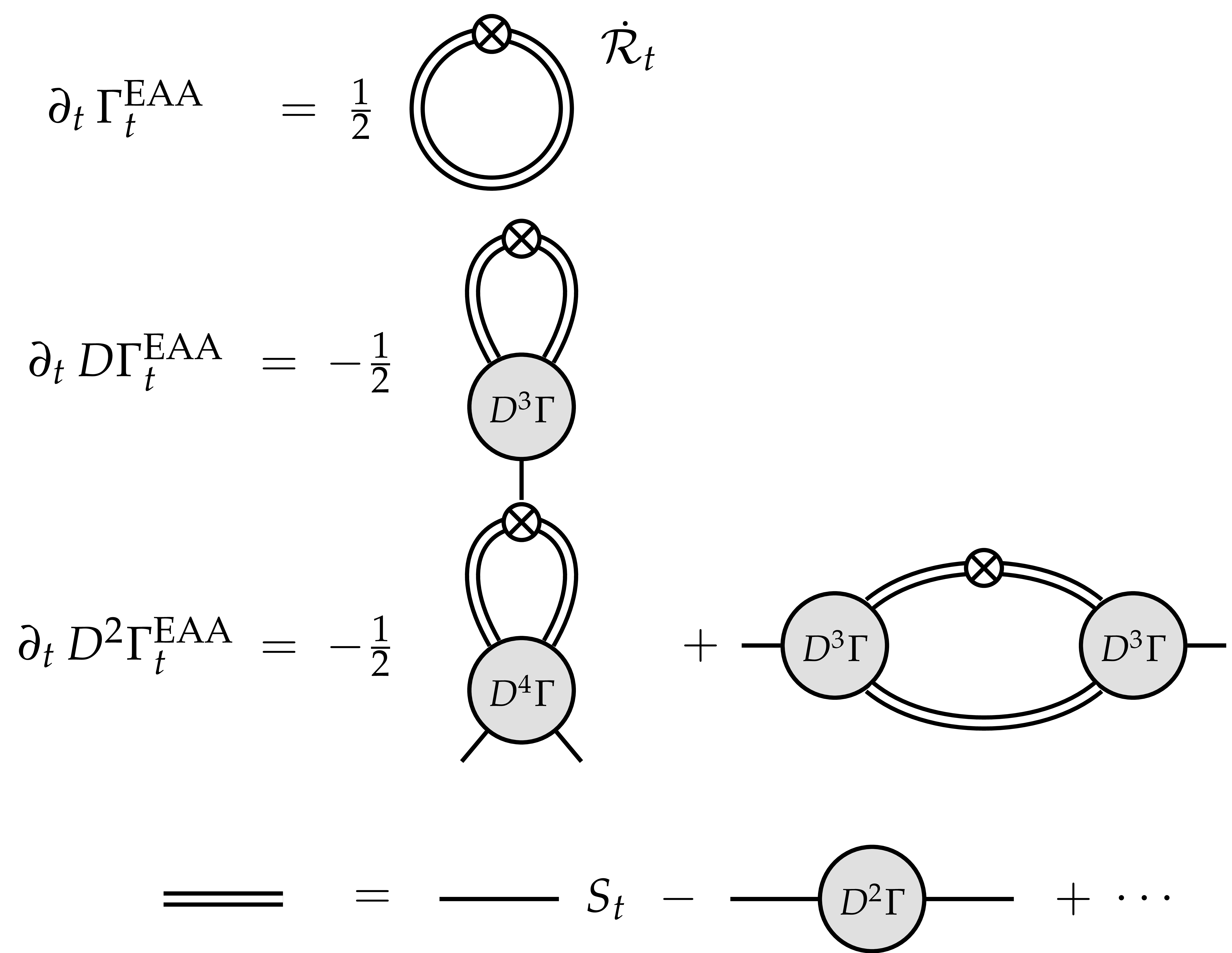
Double line: full response. Cross: \(\dot{\mathcal{R}}_t\). Exactly one loop: the Legendre transform has absorbed the tree term.
Every object in the Wetterich equation is an observable of the Polchinski process.
| Wetterich | FBSDE |
| field argument \(\psi\) | forecast \(\psi_t =\mathbb{E}_t [\Phi_T]\) |
| \(\mathrm{D} \Gamma_t (\psi_t)\) | minus the costate, \(\mathbb{E}_t [\mathrm{D} V_T (\Phi_T)]\) |
| propagator \((\mathrm{D}^2 \Gamma^{\text{EAA}}_t +\mathcal{R}_t)^{- 1}\) | conditional covariance \(\text{Cov}_t\) |
| regulator \(\mathcal{R}_t = S_t^{- 1} - Q_T^{- 1}\) | shell precision minus prior precision |
| \(\partial_t \Gamma_t\) | \(\frac{1}{2} \text{Tr} [\dot{\mathcal{R}}_t (\text{Cov}_t - S_t)]\) |
Driven by interacting minus free conditional covariance; one-loop exact, with the full propagator; in the Gaussian case only the constant flows. Wetterich 1993; Morris 1994; Berges–Tetradis–Wetterich 2002
Value function. At the optimal forecast, \(V_t (x) = \Gamma_t (\psi) +\mathcal{A}_t (x, \psi)\): the cost attached to the forecast plus the cost of reaching it by free motion. This transports the generating function along \(\Sigma_t\):
Legendre. With \(\mathcal{K}_t (S_t^{- 1} x) = \frac{1}{2} \langle x, S_t^{- 1} x \rangle - V_t (x)\) up to a function of \(t\),
\(V_t\) in the field \(x\); \(\mathcal{K}_t\) in the coordinate \(j = S_t^{- 1} x\); \(\Gamma_t\) in the forecast \(\psi\).
Polchinski is the Hamilton–Jacobi equation of \(\mathcal{K}\); Wetterich is its Legendre dual. The regulator is the information gained.
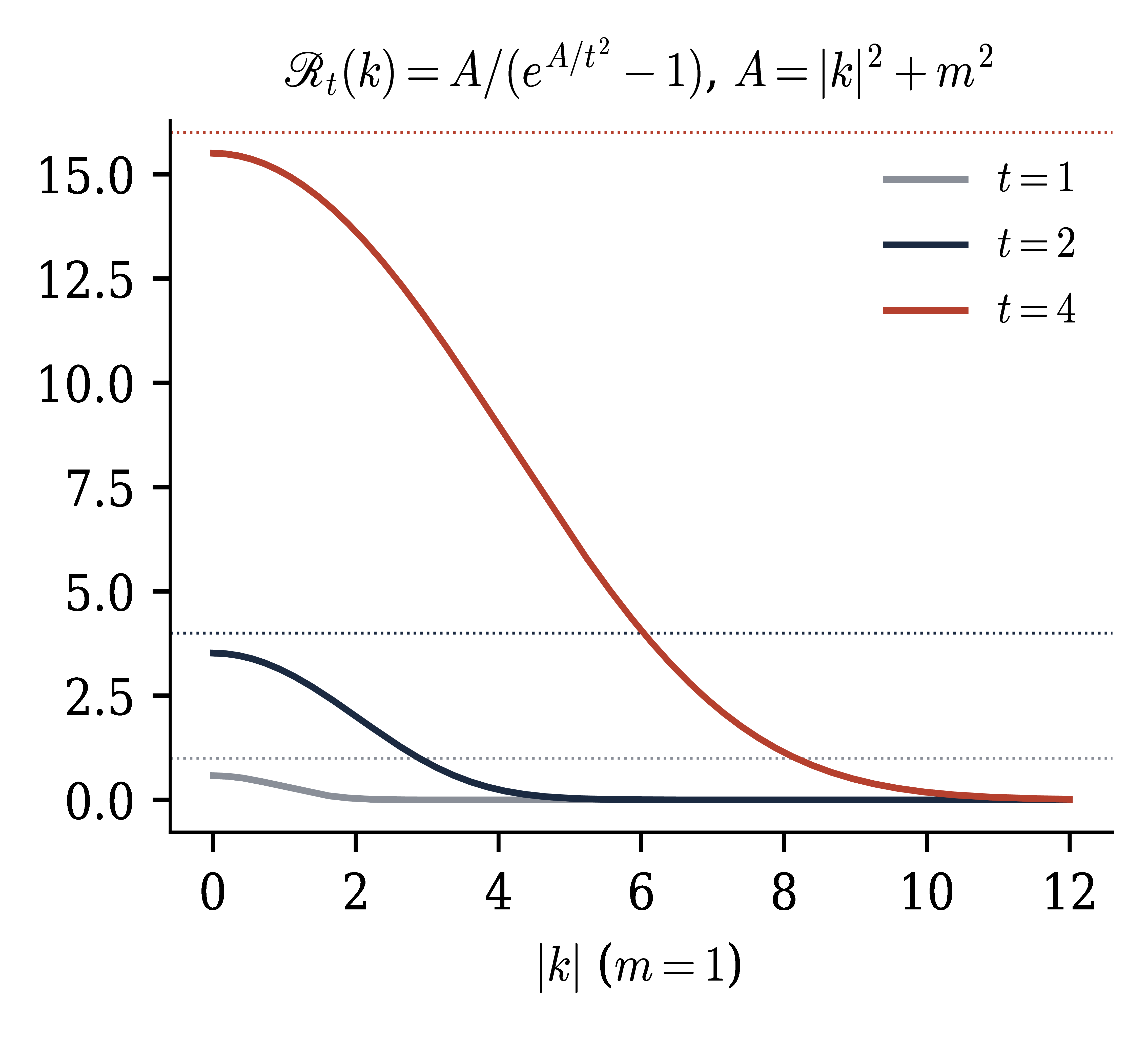
For \(T = \infty\), \(S_t = C (1 - \mathrm{e}^{- A / t^2})\) and
The exponential regulator of the functional RG. Other profiles give other regulators, e.g. the mass regulator \(\mathcal{R}_t = t^2\). |
|
At \(t = 0\): the 1PI effective action of \(\nu_T\) (Jona-Lasinio 1964),
Cramér: the mean of \(N\) independent samples is \(\approx \psi\) with probability \(\approx \mathrm{e}^{- N (\Gamma^{\text{EAA}}_0 (\psi) - V_0 (0))}\): a large-deviation rate function.
Convex even when \(V_T\) is not; minimal at the mean; Hessian there \(=\) inverse covariance.
Formally, the same for the field averaged over a large volume: \(\Gamma\) per unit volume (the effective potential of QFT, not \(V_t\)) is the rate function of the magnetisation; flat parts may appear (Maxwell).
The renormalisation group as a probabilistic object: limit theorems for strongly dependent variables.
Jona-Lasinio, Nuovo Cimento 1964; Nuovo Cimento B 1975; Phys. Rep. 2001.
Constrained free energy. Gibbs variational principle for the conditional law:
the free energy of the unresolved shell, constrained to the forecast. \(V_t\) is the value function; \(\Gamma_t\) is its Moreau transform.
Tree level. Drop the Itô term: \(\Gamma_t = V_T\), and the Moreau transform becomes the Hopf–Lax formula
which solves \(\partial_t V = \frac{1}{2} \langle \mathrm{D} V, \dot{Q} \mathrm{D} V \rangle\): the saddle point of the Gaussian convolution. The minimiser solves the classical field equation \(S_t^{- 1} (y - x) + \mathrm{D} V_T (y) = 0\) in the shell \([t, T]\); expanding in \(V_T\) gives exactly the tree diagrams.
Three constructions of the interacting measure, renormalisation, control and filtering, produce one forward–backward system. Backward in resolution it is a linear Gaussian blurring of \(\nu_T\).
In force coordinates the system has no drift, trees are integrated exactly, and the propagator is the conditional covariance.
Potentials: the value function generates the canonical transformation to these coordinates; the Legendre transform of the filter gives \(\Gamma_t\) and the Wetterich equation.
Next
Lecture 5: observables, the field equation at every resolution and its sub-Gaussian noise.
Exercises (numbering of the notes)
|
Reading
|