Constructive quantum field theory — Lecture 5 (slides)

Minkowski (Lecture 1): \((\Box + m^2) \varphi + V' (\varphi) = 0\) as an operator equation, with the CCR. On time-ordered functions \(\partial_t^2\) also hits the step functions:

Contact terms: the canonical commutator, a derivative, \(\mathrm{i} [\partial_t \varphi (\textbf{x}), \cdot] = \delta / \delta \varphi (\textbf{x})\). Rotate, \(t = - \mathrm{i} \tau\): \(\Box + m^2 \to A\), \(- \mathrm{i} \delta (t) \to \delta (\tau)\), and we get the DS equation of Lecture 2:

nonzero: the Euclidean field does not solve \(A \varphi + V' (\varphi) = 0\).

Nelson (1975): condition in real space. On the lattice \(\varepsilon \mathbb{Z}^d\), \(\omega := A \varphi + V' (\varphi)\). By the Markov property \(\varepsilon^d \omega (x)\) is minus the score of the law of \(\varphi (x)\) given its neighbours:

not Gaussian. A random variable iff \(\mathbb{E}V'' (\varphi) < \infty\) in the limit (heuristically): unlikely in \(d = 3\) (cf. Albeverio–Liang–Zegarlinski 2006). \(\omega\): Nelson's Euclidean noise (we keep his letter); as far as we know, not studied since as a noise.

Albeverio–Yoshida (2002): prescribe a Gaussian noise. Solve \(A \psi + V' (\psi) = A^{1 / 2} \xi\): \(\psi + A^{- 1} V' (\psi)\) is a free field, and formally

nonlocal, not Markov, no reflection positivity (only on functionals of \(\psi + A^{- 1} V' (\psi)\), a free field).

Substitute \(\Phi_t = \psi_t - S_t F_t\); since \(KS_t = 1 - J_t\), the smoothing disappears: \(K \psi_t = F_t + \omega_t\). As \(T \to \infty\), with \(F_t = - \mathrm{D} \Gamma_t (\psi_t) = - \mathrm{D} V_t (\Phi_t)\):

• For the forecast the force acts on the same variable, with no smoothing: the Euler–Lagrange equation of \(\frac{1}{2} \langle \psi, A \psi \rangle + \Gamma_t (\psi)\), forced by \(\omega_t\).

• \(\Phi^4\), one loop (finite \(T\), first order in \(\lambda\)): \(\Gamma_t \approx V_T + \frac{1}{2} \text{Tr} (S_t \mathrm{D}^2 V_T)\) moves the Wick ordering to \(c_t\):

  \(\displaystyle \langle \psi_t, K \psi_t \rangle + \frac{\lambda}{3} \int (\psi_t^4 - 3 c_t \psi_t^2) = \langle \psi_t, \omega_t \rangle + \ldots,\)

  and \(a^4 - 3 c_t a^2 \geqslant \frac{1}{2} a^4 - \frac{9}{2} c_t^2\) (since \((a^2 - 3 c_t)^2 \geqslant 0\)): the coercivity of the cube is visible (heuristically; in \(d = 3\) the mass counterterm still diverges). For \(\Phi_t\) it is hidden behind \(\mathrm{e}^{- A / t^2}\).

• IBP: \(\mathbb{E} [G (\psi_t) \langle h, K \psi_t - F_t \rangle] =\mathbb{E} [\mathrm{D}_{\text{Cov}_t \mathcal{R}_t h} G (\psi_t)]\).

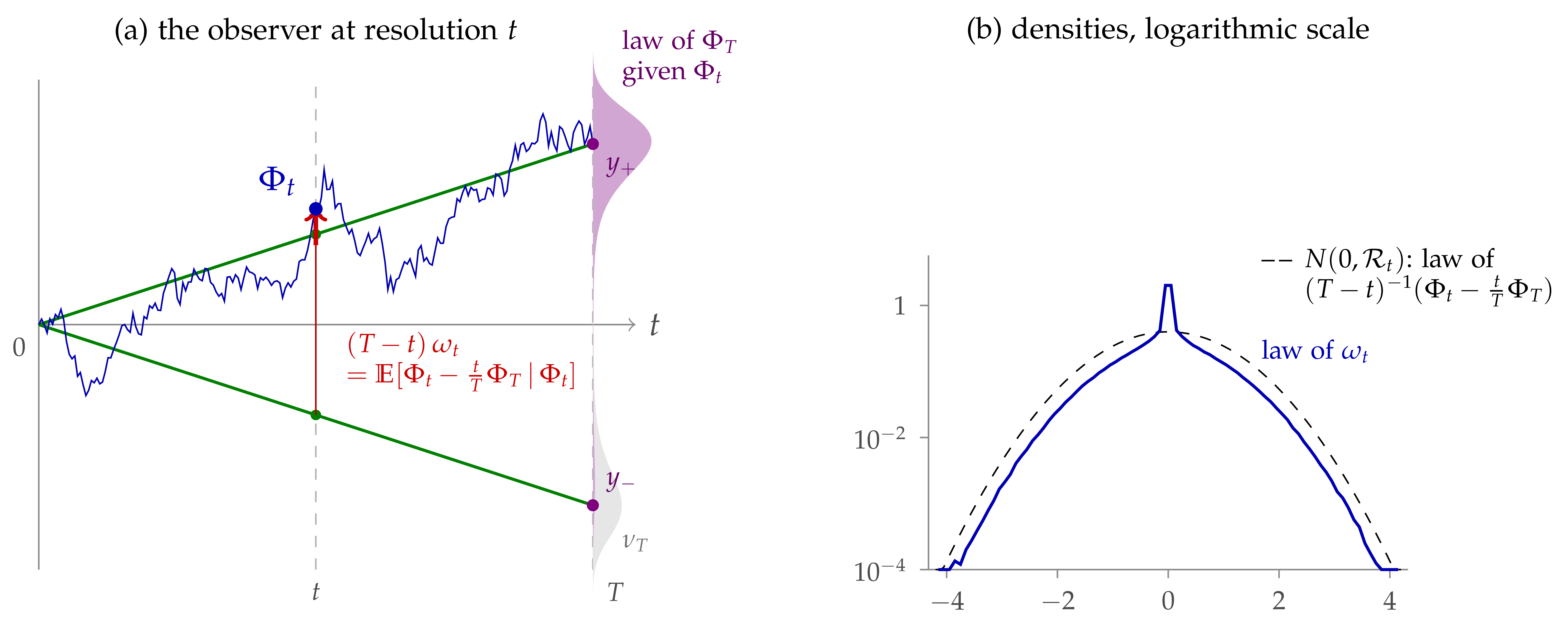
One mode, \(Q_t = t\). Known endpoint \(y\): a Brownian bridge, \(\Phi_t = \frac{t}{T} y + \zeta_t\) and \(\omega_t = \zeta_t / (T - t) \sim N (0, \mathcal{R}_t)\). Random endpoint \(\Phi_T \sim \nu_T\): \(\omega_t =\mathbb{E} [(\Phi_t - \frac{t}{T} \Phi_T) / (T - t) | \Phi_t]\).

\(T = 1\), \(t = 1 / 2\), \(\nu_T (\mathrm{d} y) \propto \mathrm{e}^{- 2 y^4 + 6 y^2} N (0, 1) (\mathrm{d} y)\) (grey). Green: bridges to the endpoints \(y_{\pm}\); violet: posterior. The peak at \(0\) in (b): a fold of \(\Phi_t \mapsto \omega_t\) between the wells.

General field: \(\text{Cov} (\omega_t) =\mathcal{R}_t - S_t^{- 1} J_t \mathbb{E} [\text{Cov}_t] J_t S_t^{- 1} = KJ_t + J_t \mathbb{E} [\mathrm{D}^2 V_t (\Phi_t)] J_t\): the free bridge noise minus what the observer cannot resolve; Nelson's mass \(m^2 +\mathbb{E}V''\), at resolution \(t\), and finite.

\(\omega_t\) is minus the score of the law of \(\Phi_t\) (density \(p_t\)), seen through \(J_t\): \(\omega_t = - J_t \mathrm{D} \log p_t (\Phi_t)\). Given \(\Phi_T\), the interacting field is still the Gaussian bridge:

\(F_t = - \mathrm{D} V_t (\Phi_t) = - \mathrm{D} \Gamma_t (\psi_t)\). Read it from the measure at resolution \(t\), \(\nu_t \propto \mathrm{e}^{- V_t} \mu^{Q_t}\).

1. Always: \(\mathrm{D}^2 V_t \leqslant S_t^{- 1}\) (\(\text{Cov}_t \geqslant 0\)), then Cameron–Martin:

   \(\displaystyle \mathbb{E} \mathrm{e}^{u \langle h, F_t \rangle} \leqslant \mathrm{e}^{\frac{u^2}{2} \langle h, (S_t^{- 1} - Q_t^{- 1}) h \rangle} \hspace{0.17em} \mathbb{E} \mathrm{e}^{u \langle Q_t^{- 1} h, \Phi_t \rangle} .\)

2. Convexity: \(\Gamma_t\) convex \(\Rightarrow\) \(V_t\) convex \(\Rightarrow\) (Prékopa) \(\Phi_t\) no wider than the free field: \(\mathbb{E} \mathrm{e}^{\langle k, \Phi_t \rangle} \leqslant \mathrm{e}^{\frac{1}{2} \langle k, Q_t k \rangle}\).

• \(\mathcal{R}_t \leqslant t^2 \mathrm{e}^{- A / 2 t^2}\): at resolution \(t\), \(\omega_t \lesssim t \times\) white noise smoothed at scale \(1 / t\), so \(\omega_t (x) = O (t^{1 + d / 2})\).

• At scale \(1 / t\) this is the size of regularity \(- 1 - d / 2\) (\(- 5 / 2\) in \(d = 3\)): one derivative rougher than white noise, like the free noise \(A^{1 / 2} \xi\), whatever the interaction.

• Not a limit distribution: on a fixed \(h\) only \(\langle h, \omega_t \rangle = O (t)\), while the free noise stays bounded.

• On resolved modes (\(|k| \ll t\)) the bound exceeds the free noise by \(t^2 / A\); it is attained by a pinning potential \(\kappa \| \varphi \|^2 / 2\), \(\kappa \to \infty\).

• Pathwise (convex domination of the norm, Doob): a.s. for \(t \geqslant 1\) (\(t \leqslant T / 2\) if \(T < \infty\)), at finite spatial cutoff, with a random constant \(\tilde{C}\),

  \(\displaystyle \sup_x (1 + |x|)^{- \delta} | \omega_t (x) | \leqslant \tilde{C} t^{1 + d / 2} \sqrt{\log (2 + t)} .\)

Perturb the optimal drift \(u^{\ast}\) of the Boué–Dupuis formula (Lecture 4), \(X^{u^{\ast}} = \Phi\): \(u = u^{\ast} + w\), \(X^u = \Phi + I (w)\), \(I_t (w) = \int_0^t \dot{Q}_s^{1 / 2} w_s \mathrm{d} s\). Euler–Lagrange gives the cross term

\(B_V (\phi, h) = V (\phi + h) - V (\phi) - \langle \mathrm{D} V (\phi), h \rangle\): the first-order Taylor remainder.

• Minimiser: \(\Phi^f = \Phi + I (w^{\ast})\) solves the FBSDE with terminal potential \(V_T + f\), a perturbation of \(\Phi\):

  \(\displaystyle F^f_s - F_s = -\mathbb{E}_s [\mathrm{D} f (\Phi^f_T) + \mathrm{D} V_T (\Phi^f_T) - \mathrm{D} V_T (\Phi_T)] .\)

Gaussian convolution lowers the Wick ordering: \(V_t = \int [\frac{\lambda}{12} : \phi^4 :_t + \gamma_T : \phi^2 :_t] + O (\lambda^2)\) (\(\gamma_T = O (\lambda^2)\), kept for later use; \(: \phi^p :_t = H_p (\phi ; c_t)\), \(c_t = Q_t (x, x)\)): dual to \(\int H_4 (X_t ; c_t)\) being an observable (Lecture 3). At second order, \(S = S_t\):

\(T \to \infty\) at fixed \(t\), \(d = 3\), \(G (z) \sim (4 \pi |z|)^{- 1}\) (the kernel of \(A^{- 1}\)):

• \(k = 1, 2\): finite, nonlocal.

• \(k = 3\) (sunset): \(S^3 \sim |z|^{- 3}\); local divergence \(- \frac{\lambda^2}{3} (\int S^3) \int : \phi^2 :_t\) (+ finite), cancelled by \(\gamma_T = \frac{\lambda^2}{3} \int Q_T^3 = \frac{\lambda^2}{48 \pi^2} \log T + O (1)\).

• \(k = 4\): vacuum energy \(\sim T\); cancels in \(\nu_T\).

Renormalisation \(=\) choosing \(V_T\) so that \(V_t\) at fixed resolution converges. \(\nu_t \ll \mu^{Q_t}\) expected for \(t < \infty\); the terminal \(\Phi^4_3\) is singular w.r.t. the GFF.

\(\rho \geqslant 0\), \(\mathbb{E}_{\nu_T} \rho = 1\), \(M_t =\mathbb{E}_t \rho (\Phi_T) = G_t (\Phi_t)\), \(G_t (\phi) = \int \rho \mathrm{d} \mu_t^{\phi}\).

• \(M_0 = 1\), \(M_T = \rho (\Phi_T)\), and \(\mathrm{d} M_t = \langle \mathrm{D} G_t (\Phi_t), \dot{Q}_t^{1 / 2} \mathrm{d} W_t \rangle\).

• Itô for \(M \log M\):

  \(\displaystyle \operatorname{Ent}_{\nu_T} (\rho) = \frac{1}{2} \mathbb{E} \int_0^T \frac{\mathrm{d} \langle M \rangle_t}{M_t} = 2\mathbb{E} \int_0^T \left\| \dot{Q}_t^{1 / 2} \mathrm{D} \sqrt{G_t} (\Phi_t) \right\|^2 \mathrm{d} t.\)

• Stopping at \(t\): revealed + hidden entropy,

  \(\displaystyle \operatorname{Ent}_{\nu_T} (\rho) =\mathbb{E} [M_t \log M_t] +\mathbb{E}\operatorname{Ent}_{\mu_t^{\Phi_t}} (\rho) .\)

• The increments see the conditional law: \(\mathrm{D} G_t (\phi) = S_t^{- 1} \operatorname{Cov}_{\mu_t^{\phi}} (\rho, y)\).

• Entropic stability (Chen–Eldan; \(\dot{\mathcal{R}}_r = S_r^{- 1} \dot{Q}_r S_r^{- 1}\)): if \(\dot{\mathcal{R}}_r \operatorname{Cov}_{\mu_r^{\phi}} \dot{\mathcal{R}}_r \leqslant \alpha_r \dot{\mathcal{R}}_r\) for all \(\phi\) and \(r \leqslant t\), then \(\operatorname{Ent}_{\nu_T} (\rho) \leqslant \mathrm{e}^{\int_0^t \alpha_r \mathrm{d} r} \mathbb{E}\operatorname{Ent}_{\mu_t^{\Phi_t}} (\rho)\): the low resolutions must not hide too much.

Bauerschmidt–Bodineau–Dagallier, Probab. Surveys 2024: their fluctuation measure is our stochastic localisation (scale reversed).

• Gradient bound at each scale + entropy formula. Gaussian check: \(V_T = 0\), \(Q_t = tQ_T / T\), \(\kappa = 0\) \(\Rightarrow\) Gaussian LSI.

• Convexity of the effective potentials, not of \(V_T\).

• By \(\mathrm{D}^2 V_t = S_t^{- 1} - S_t^{- 1} \operatorname{Cov}_t S_t^{- 1}\), for \(\dot{Q}_t\) invertible the hypothesis is equivalent to the bound, uniform in \(\phi\),

  \(\displaystyle \operatorname{Cov}_t \leqslant S_t - S_t \dot{Q}_t^{- 1} \left( \kappa_t \dot{Q}_t - \frac{1}{2} \ddot{Q}_t \right) \dot{Q}_t^{- 1} S_t :\)

  at most \(S_t\) iff \(\kappa_t \dot{Q}_t \geqslant \frac{1}{2} \ddot{Q}_t\) (linear profile: \(\kappa_t \geqslant 0\)).

• Bridge: \(\mathrm{D}^2 V_t = S_t^{- 1} - S_t^{- 1} \operatorname{Cov}_t S_t^{- 1}\): convex potentials \(=\) bounded conditional covariance.

• Bauerschmidt–Bodineau: Bakry–Émery for the Kolmogorov equation, curvature \(\dot{Q} \mathrm{D}^2 V_t \dot{Q} + \frac{1}{2} \ddot{Q}\): gradient bound at each scale, LSI at the terminal scale, far from log-concavity. Uniform in \(\phi\): suits the RG (sine-Gordon, \(\beta < 6 \pi\)).

• Localisation: bound what is lost on \([0, t]\), then use a known inequality for \(\mu_t\). Moments of the conditional law, possibly only with high probability (KLS).

Bauerschmidt–Bodineau, CPAM 2021; Bauerschmidt–Bodineau–Dagallier, Probab. Surveys 2024; Eldan, GAFA 2013; Chen–Eldan, FOCS 2022.