|
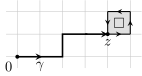
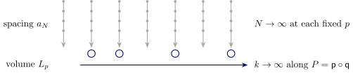
Figure 1. The two limits of Definition 2.6. At every fixed volume the full sequence of spacings is used (vertical arrows); the volume limit then runs along the retained indices \(P (k)\) (circled), chosen once for all fields and tests. |
|
Abstract
For every closed subgroup \(G \subset U (n_G)\) with simple nonabelian Lie algebra \(\mathfrak{g}\) and every positive block penalty, the coefficient of the soft constraint that ties each coarse link to a predictor computed from the fine transports, we construct gauge-invariant local fields from four-dimensional Wilson measures. Exact scale integration and tuning to a common endpoint coupling give the full ultraviolet limit at fixed volume. Reflection positivity and chessboard bounds give volume-uniform control; compactness gives a limit along a refinement of any prescribed strictly increasing volume sequence. The limit decomposes into phases, each the Euclidean continuation of a faithful Wightman theory with unique vacuum. The fields carry a conserved stress tensor, an operator product expansion with spectator-independent coefficients and phase-uniform remainders, and distributional extensions through collisions. In a selected phase, the centered stress trace has a two-point function \(G_{\Theta}\) with \(r^8 \log^2 (1 / r) \hspace{0.17em} G_{\Theta} (r) \to 3 \dim_{\mathbb{R}} \mathfrak{g}/ \pi^4\) as \(r \downarrow 0\), and on no interval \((0, \delta)\) does \(G_{\Theta}\) agree with a finite Wick profile, a finite sum of products of free mass-shell Laplace kernels. No mass gap, uniqueness of the volume limit or phase, or independence from the block penalty is proved.
This paper was written entirely by AI agents from OpenAI's Lean code for the construction of four-dimensional quantum Yang–Mills theory (commit 3456e5e). The Lean proof is kernel-checked, with only the standard axioms. The agents compared every numbered statement here with the Lean declarations used by the main theorem; the correspondence table is published separately. The prose arguments were written and reviewed by AI agents. They are not machine-checked and have not been refereed by human mathematicians (Section 1.1).
IThe theorem and the architecture of its proof 5
1The result 5
Main result. 6
What is not claimed. 7
1.1Source of the result and of this text 7
1.2Earlier work and the method 7
1.3Reading guide 9
1.4Notation and conventions 9
2Definitions 10
2.1The gauge group and the Wilson measure 10
2.2Wilson families and their correlations 11
2.3Local fields 13
2.4Euclidean properties 15
2.5Field spaces and phases 16
Phases. 16
2.6Wightman theories 16
2.7The trace and product statements 17
3The main theorem 18
Order of choices. 19
What the theorem does not assert. 19
4Strategy of the proof 20
4.1Why the ultraviolet induction closes 21
One coupling to tune. 21
The scales. 21
The cancellations. 21
Large fields. 23
Growing block ratios. 23
4.2Tuning, uniqueness and convergence 23
4.3Rotations 24
4.4Phases and reconstruction 25
4.5The trace 25
5The renormalization group 26
5.1Scales and the block map 26
5.2The density and its norms 28
5.3The inductive step 31
5.4Multiscale trajectories 32
5.5Local fields under blocking 34
5.6Uniform bounds and the fixed-volume limit 35
6The continuum limit, stress, phases, trace and products 36
6.1The volume limit and the field calculus 36
6.2Stress and rotations 38
6.3Phases and reconstruction 41
6.4Trace and products 43
7Deduction of the main theorem 46
8Correspondence with the formal statement 47
8.1Hierarchy data and the conditions Q0–Q6 48
8.2Formal conventions 49
8.3An averaged countertest 50
9Constants and order of choice 50
Index of notation 52
IIProofs 55
10Local polynomial fields 55
10.1Labels, test holonomies and the Taylor map 56
10.2Taylor-normalized sections 57
10.3Small-field bounds 59
10.4Auxiliary equation sections 60
Idea: free equations in an interacting theory. 61
Lattice symmetries. 61
10.5Example: the curvature square 64
The label. 64
Two lattice readings. 65
The insertion. 65
The field. 65
11Gauges and block integration 66
Induction scheme. 66
11.1The block kernel 67
Measurability and covariance of the block kernel. 70
11.2Free quadratic forms 70
11.3The stationary background and Gaussian coordinates 75
Tree gauge. 75
Block norms. 76
Gaussian coordinates. 79
11.4Inverse, vertex and Ward estimates 80
The regulator. 80
The predictor contact term. 81
The compared operators. 81
Insertion bounds. 82
Vertices. 84
The stationary Ward identity. 87
11.5The local large-field energy 88
Square completion. 89
Selections. 90
11.6Sector Gaussian integration 95
The differentiated local integral. 98
Factors and their bounds. 99
The reference law and the transported integrand. 100
12Path actions and the one-loop coupling 105
12.1Curvature coordinates and the path action 106
12.2Fourth-order matching 108
A finite-dimensional model. 110
12.3The determinant comparison 111
12.4The one-loop coefficient 114
13Activities and the inductive step 118
Local terms and their norms. 118
Coefficient algebras. 120
Support exponents. 120
13.1The local expansion 121
Ordinary or forced: an example. 122
One factor followed to the output allowance. 127
13.2Local quadratic subtraction 137
13.3Forced fusion, activity bounds and the reset 139
The scalar reset. 143
13.4Continuity at fixed volume 145
13.5The Wilson start 146
13.6The specified recursion 149
13.7Weighted analytic estimates 150
What is held fixed. 150
14Trajectories, marked fields and ultraviolet convergence 161
14.1Trajectories and tuning 162
14.2Marked fields and volume-uniform estimates 169
14.2.1One marked insertion 169
The curvature square at the terminal map. 174
14.2.2Chessboard seminorms and replicated sources 176
Replicated sources. 177
14.2.3Negligible errors and local matching 183
14.2.4Equation identities and coefficient corrections 186
14.2.5Comparison with free fields 188
Comparison windows. 190
14.2.6Bounds for lattice differences 197
14.2.7Bounded approximations 200
14.3Full ultraviolet convergence 203
15Infinite volume and field calculus 210
15.1Volume limits 210
Symmetries of the limit. 211
15.2Separated cells and negligible errors 211
15.3Quotient fields 212
Example: the curvature square (continued). 215
15.4Euclidean properties 215
15.5Repeated reflected words 216
16Free fields, Ward identities and rotations 218
16.1Free fields 219
16.2Lattice inputs 226
16.3Free comparison and the conserved line 231
16.4Coordinate reflection spaces and spectral estimates 234
16.5Ward identities and rotations 240
17Phases and reconstruction 246
17.1Compression and phases 247
17.2Reconstruction 252
18The trace law and non-free comparisons 259
18.1Trace and spectrum 259
Comparison at prescribed radii. 261
Tensor coordinates. 263
Lattice stress current. 264
Block transfer. 264
Extraction of the scalar coefficient. 265
A stability lemma. 268
Transfer to the continuum. 268
Why a rate is needed. 268
18.2Precise non-free comparisons 275
19Products and contact subtractions 279
Inputs from the marked expansion and the quotient. 280
19.1Products and nested clusters 284
19.2Contact subtractions 296
Two scales. 300
References 304
IThe theorem and the architecture of its proof
How can a lattice model give a quantum field theory in continuous space-time? We answer this question for four-dimensional Yang–Mills theory with a compact gauge group whose Lie algebra is simple and nonabelian, starting from Wilson's lattice gauge theory [36]. On a finite periodic lattice the variables are group elements attached to the links, and their law is an ordinary probability measure. Let \(G \subset U (n_G)\) be a closed matrix group, \(s \geqslant 1\) an integer and \(\Lambda_s = (\mathbb{Z}/ s\mathbb{Z})^4\). A configuration assigns \(U (y, a) \in G\) to the positive link from the site \(y\) in the coordinate direction \(a\), and \(U (y, a)^{- 1}\) to the reversed link. For \(\beta \in \mathbb{R}\),
where \(dh\) is probability Haar measure and \(Z_{s, \beta}\) normalizes the measure. The plaquette holonomy \(U_{y ; ab}\) is the transport around an elementary square, and \(\beta\) penalizes its distance from the identity. The problem is to choose the inverse coupling and the local observables as functions of the lattice spacing so that their correlations converge as the spacing tends to zero and the volume grows, and to identify the limit. No measure on continuum connections is constructed here. What converges are the correlations of gauge-invariant local observables at distinct points; the continuum theory is the resulting family of correlation functions, from which Hilbert spaces and relativistic quantum fields are then reconstructed.
| \(\displaystyle \frac{\beta_{N, p}}{\log (1 / a_N)} \longrightarrow \kappa_G = \frac{11 C_{\mathfrak{g}}}{24 \pi^2} \qquad (N \to \infty), \quad \text{uniformly in } p \hspace{0.17em}, \) | (1.2) |
where \(C_{\mathfrak{g}}\) is the adjoint Casimir in the trace normalization of Definition 2.1 (for \(SU (n)\), \(\kappa_G = 11 n^2 / (12 \pi^2)\); Remark 2.2). The family has the following properties; Theorem B in Section 3 states them precisely.
At each fixed volume, correlations of the insertions, smeared against smooth tests supported away from coincident points and inside one period cell, converge along the full sequence of spacings.
Every prescribed strictly increasing sequence \(\textsf{p}\) of volume indices has a strictly increasing refinement \(\textsf{q}\) such that, with \(P = \textsf{p} \circ \textsf{q}\) and the lattice correlations \(C^{\text{lat}}_{N, p}\) of Definition 2.4,
| \(\displaystyle \lim_{k \to \infty} (\lim_{N \to \infty} C^{\text{lat}}_{N, P (k)} (v ; f)) = \int f (x) S_n (v ; x) \hspace{0.17em} dx\) | (1.3) |
for one table \(S\) of Euclidean correlation functions, symmetric under permutations, translations and signed permutations of the axes, reflection positive, smooth away from collisions and polynomially bounded near them (properties E1–E7 of Section 2.4). One refinement serves all insertions and all tests.
\(S = \int_{\textsf{X}} S^{\xi} \hspace{0.17em} d \nu (\xi)\) is an average of phases over a compact metric space with a fully supported probability measure, and each \(S^{\xi}\) is the Euclidean continuation of a faithful Wightman theory with unique vacuum.
The fields carry a conserved symmetric stress tensor, normalized by its action on the other fields. In a selected phase, the two-point function \(G_{\Theta}\) of the centered trace of this tensor satisfies
| \(\displaystyle \lim_{r \downarrow 0} r^8 \log^2 (1 / r) \hspace{0.17em} G_{\Theta} (r) = \frac{3 \dim_{\mathbb{R}} \mathfrak{g}}{\pi^4} > 0 \hspace{0.17em},\) | (1.4) |
and on no interval \((0, \delta)\) does \(G_{\Theta}\) agree with a finite Wick profile, a finite sum of finite products of free mass-shell Laplace kernels (Definition 2.18).
Nearby fields have an operator product expansion whose coefficients depend neither on the other fields nor on the phase, with remainders bounded uniformly in the phase. The correlations of each phase extend across coincident points by an explicit subtraction of Taylor jets.
Theorem B holds for every \(\textsf{b} > 0\). Section 8 states the existence theorem in the exact form of the formal statement (Theorem A), which asks only for some positive logarithmic slope, and deduces it from Theorem B.
The mathematical result is due to OpenAI's Lean construction at commit 3456e5e of the repository yang-mills-group/OpenAI-YM-20261028 [24]. Theorem B records that construction; Section 8 states its top-level existence theorem and deduces it. Three kinds of checking are involved, and they should be kept apart.
The Lean kernel checks the formal proof. Its kernel-check record reports no unproved placeholders in the proved theorem and only propositional extensionality, classical choice and quotient soundness as axioms.
AI agents compared every numbered statement of this text with the Lean declarations used by the main theorem: hypotheses, definitions, quantifier order, normalizations and conclusions, with usage determined from the compiled dependencies. The correspondence table is published separately; the source repository supplies a declaration-usage table.
The prose arguments were written and reviewed by AI agents. They are not machine-checked and have not been refereed by human mathematicians.
A correct formal declaration does not by itself show that an English statement has kept its hypotheses and quantifiers, or that a prose proof proves that statement. This text was written entirely by AI agents under human direction, with separate writing and checking of statements and arguments, by the method described in How the manuscript is written. The work is carried out in collaboration with Martin Hairer's humanise-yang-mills project.
Table 1 lists, for the main mechanisms of the proof, the closest earlier rigorous result and its use here. The comparison concerns how these operations are combined; it assigns none of them a new origin, and we make no priority claim for renormalization-group principles or physical predictions.
|
||||||||||||||||||||||||||||||
The renormalization group is organized as in the method of Bauerschmidt, Brydges and Slade [6]: an explicitly defined map, a finite-dimensional flow of couplings, norms in which the remaining coordinate contracts, and a global trajectory with a tuned initial parameter. What requires proof here is the compatibility of the one-loop slope with the exact gauge block map, the coupling reset and the tuning to a common endpoint, followed by continuum identifications on one family: control of composite fields, restoration of rotations through stress-tensor fluxes, the trace law through all radii and product bounds uniform over phases.
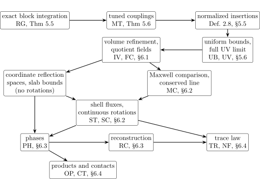
Section 2 defines the objects needed to state Theorem B, which is Section 3. Section 4 explains the route of the proof and the mechanisms that make it work, with a dependency map (Figure 2). Sections 5 and 6 state the principal results, each with the idea of its proof, and Section 7 deduces Theorem B. Part II gives the proofs. Table 2 lists the principal results; their tags appear in statement titles. Section 9 records the order in which constants are chosen. A first reading can skip the coordinates of the effective densities (Section 5.2), the marked decomposition (Section 5.5) and Section 9. The index of notation follows the appendices.
|
||||||||||||||||||||||||||||||||||||||||||||||||||||||||||||||||
Throughout, \(\mathbb{N}= \{0, 1, \ldots\}\), coordinate indices run from \(1\) to \(4\), \(e_a\) is the \(a\)th coordinate vector, and time is the fourth coordinate. For the relativistic statements write
Inner products are antilinear in the first variable, and spacetime integrals use Lebesgue measure. Correlations of arity zero are included; empty sums are zero and empty products are one. The group \(H_4\) consists of the signed permutation matrices, and \(\textsf{s}_a^{\text{refl}}\) denotes reflection in the \(a\)th coordinate.
This section defines the objects needed to state the main theorem: the gauge group and the Wilson measure, families of lattice theories and the convergence of their separated correlations, the local fields, the Euclidean properties of the limit, its field spaces, Wightman theories, and the quantities of the trace and product statements. The renormalization-group objects that construct the family are defined in Section 5, where they are used.
The matrix normalization fixes both the Wilson energy and the coefficient of the logarithmic coupling flow.
Definition
For an orthonormal basis \((e_{\alpha}^{\mathfrak{g}})\), put
Here \(\text{ad} (X) Y = [X, Y]\) and \(\text{tr}_{\mathfrak{g}}\) is the real operator trace on \(\mathfrak{g}\). Simplicity means \([\mathfrak{g}, \mathfrak{g}] \ne 0\) and no proper nonzero real ideal; connectedness of \(G\) is not assumed. The adjoint maps are skew-adjoint for this metric, so nonabelianity gives \(C_{\mathfrak{g}} > 0\) and \(\kappa_G > 0\). For \(u \in G\) the plaquette energy and the normalized chord are
both are invariant under conjugation and inversion, and the chord measures the distance of a plaquette holonomy from the identity.
Remark
Definition
The integrand of \(Z_{s, \beta}\) is continuous and strictly positive on the compact configuration space, so \(0 < Z_{s, \beta} < \infty\). The link variable \(U (y, a)\) carries a row vector \(\psi \in \mathbb{C}^{n_G}\) at \(y\) to \(\psi U (y, a)\) at \(y + e_a\), and the ordered product along a nearest-neighbour path \(y_0, \ldots, y_k\), with inverses on reversed links, carries row vectors from \(y_0\) to \(y_k\). A site gauge transformation \(\gamma_{\text{g}} : \Lambda_s \to G\) changes the frame at each site, \(\psi \mapsto \psi \gamma_{\text{g}} (y)^{- 1}\), and acts on links by \(U^{\gamma_{\text{g}}} (y, a) = \gamma_{\text{g}} (y) U (y, a) \gamma_{\text{g}} (y + e_a)^{- 1}\). In the product along a path the intermediate factors \(\gamma_{\text{g}} (y_i)^{- 1} \gamma_{\text{g}} (y_i)\) cancel, so the product is multiplied by \(\gamma_{\text{g}} (y_0)\) on the left and \(\gamma_{\text{g}} (y_k)^{- 1}\) on the right: only the endpoints remain. Around a plaquette the path closes:
Hence the energy is gauge invariant, and invariance of Haar measure under left and right multiplication makes the measure gauge invariant. The size of a single link variable therefore carries no gauge-invariant information: the configuration \(U (y, a) = \gamma_{\text{g}} (y) \gamma_{\text{g}} (y + e_a)^{- 1}\), the transform of the identity configuration, has links far from \(1\) when \(\gamma_{\text{g}}\) varies rapidly, yet every plaquette holonomy equals \(1\). Fields are measured by gauge-invariant quantities such as plaquette chords. For a smooth \(\mathfrak{g}\)-valued field \(\mathcal{A}\) and links \(U (y, a) = \exp (h_{\text{lat}} \mathcal{A}_a (h_{\text{lat}} y))\) at a small spacing \(h_{\text{lat}}\), expansion to second order gives
the deviation of the plaquette holonomy from \(1\), divided by the enclosed area \(h_{\text{lat}}^2\), tends to the curvature, and \(\text{ch} (U_{y ; ab}) = h_{\text{lat}}^2 |F_{ab} (h_{\text{lat}} y) |_{\mathfrak{g}} + O (h_{\text{lat}}^3)\) in the norm of Definition 2.1. The measure is also invariant under the lattice isometries \(x \mapsto hx + b\), \(h \in H_4\), which transport links and invert reversed ones (Section 10.4).
A Wilson family, indexed by \(N, p \in \mathbb{N}\), consists of strictly increasing positive integer sequences \((D_N)\) and \((L_p)\), real couplings \(\beta_{N, p}\), a set \(\mathcal{T}\) of insertion labels, and complex insertions \(I_{N, p} (v, y ; U)\), functions of the configurations on \(\Lambda_{L_p D_N}\) for \(v \in \mathcal{T}\) and sites \(y\). The index \(N\) controls the spacing and \(p\) the physical volume:
| \(\displaystyle a_N = D_N^{- 1}, \qquad \mu_{N, p} = \mu_{L_p D_N, \beta_{N, p}}, \qquad \hat{y} = a_N (r_{L_p D_N} (y^a))_{a = 1}^4 \hspace{0.17em},\) | (2.2) |
where \(r_s (j)\) is the integer representative of \(j \in \mathbb{Z}/ s\mathbb{Z}\) in \((- s / 2, s / 2]\). The lattice has \(L_p D_N\) sites per side at physical distance \(a_N\), so its physical side is \(L_p\); \(\hat{y}\) places a site in the centered period cell.
Definition
The moment is the expectation of a product of insertions; the smeared correlation is its Riemann sum against a test, the factor \(a_N^{4 n}\) being the lattice volume element. The main theorem concerns a family with the following regularity.
Definition
The physical diameter of the stencil \(y + \Sigma_v\) tends to zero with \(a_N\), so the insertions are local. Condition (c) is a logarithmic growth law for the bare inverse coupling, uniform in the volume.
Correlations are tested on separated configurations. For positions in \((\mathbb{R}^4)^n\) put
with \(\text{sep}_{\infty} (x) = + \infty\) for \(n \leqslant 1\). A separated test is a smooth function on \((\mathbb{R}^4)^n\) with compact closed support in \(\text{Conf}_n\); it need not be a product of one-point tests. It is \(p\)-admissible, or supported inside volume \(p\), if its support lies in \(((- L_p / 2, L_p / 2)^4)^n\). The following definition keeps the order of the two limits explicit.
Definition
The inner limit uses the full sequence of spacings at every volume containing the support of the test; only the outer limit runs along \(P\). At volumes not containing the support, \(C_p^{\text{UV}}\) is unconstrained. In Theorem B the same \(P\) serves every arity, list of labels and test (Figure 1).
|
|
Figure 1. The two limits of Definition 2.6. At every fixed volume the full sequence of spacings is used (vertical arrows); the volume limit then runs along the retained indices \(P (k)\) (circled), chosen once for all fields and tests. |
Two examples orient this subsection. The unit label has the constant insertion one at every sufficiently fine cutoff. The curvature square \(c_{F^2} = \frac{1}{4} \sum_{a, b} \langle F_{ab}, F_{ab} \rangle_{\mathfrak{g}}\), the Yang–Mills density at a point, is read to leading order by the clover average \(P^{\text{cl}} = \frac{1}{4} \sum_{\square} \text{pr} (U_{\square})\) over the \(24\) plaquettes with a corner at the site: since \(\text{pr} = \frac{1}{2} \text{ch}^2\), the expansion of Section 2.1 gives each of them \(\frac{1}{2} h_{\text{lat}}^4 |F_{ab} |_{\mathfrak{g}}^2 + O (h_{\text{lat}}^5)\) for the links of a smooth field, so \(P^{\text{cl}} = h_{\text{lat}}^4 c_{F^2} + O (h_{\text{lat}}^5)\) with \(F\) taken at the site. The construction itself uses the local sections below, normalized by a linear map (Definition 2.8).
In general, local fields are labelled by invariant polynomials in the Taylor coefficients of a connection. The labels use radial, or Fock–Schwinger, gauge, in which the radial component of the connection vanishes. In this gauge a smooth connection satisfies \(\mathcal{A}_a (x) = \int_0^1 t \hspace{0.17em} x^b F_{ba} (tx) \hspace{0.17em} dt\), so its homogeneous part of degree \(k + 1\) is determined by the \(k\)th Taylor coefficients of the curvature at the origin.
Definition
with fixed bihomogeneous bases \(b_{d, i}\) of bidegree \((w_i, k_i)\), the supremum coefficient norm, conjugation and the induced \(H_4\) action.
For instance, at \(d = 4\) the retained part is \(\mathcal{A}_0 +\mathcal{A}_1 +\mathcal{A}_2\): for a smooth connection in radial gauge, with the curvature and its derivatives taken at the origin and repeated indices summed,
so the labels in \(V_4\) are invariant polynomials in the curvature and its first two derivatives at the origin. Curvature has weight two and each derivative adds one; for instance \(c_{F^2}\) has bidegree \((4, 2)\). Three gradings play different roles below:
the engineering weight \(w\) fixes the power of the spacing in the
Taylor normalization
the factor count \(k\) fixes the scaling by the small-field threshold, through the operator \(\textsf{N} b_{d, i} = k_i b_{d, i}\) and \(t^{\textsf{N}} b_{d, i} = t^{k_i} b_{d, i}\);
the degree \(d\) of the space \(V_d\) fixes the factor \(\ell_m^d\) in the transfer of insertions under blocking and the physical prefactor \(a_N^{- d}\).
A polynomial of weight at most \(d \leqslant e\) lies in \(V_d\) and in \(V_e\); its two insertions differ, since the normalization below depends on the degree.
Lattice holonomies are compared with smooth connection jets. For \(\textsf{j} = (\mathcal{A}_k)_k \in \mathcal{J}\), put \(\mathcal{A}^{\leqslant d} = \sum_{k + 2 \leqslant d} \mathcal{A}_k\). The test holonomies at spacing \(h_{\text{lat}}\) are, on a positive link \((y, a)\) with \(y \in \mathbb{Z}^4\),
and the jet dilation is \(\text{sc}_{h_{\text{lat}}} \textsf{j} = (h_{\text{lat}}^{k + 2} \mathcal{A}_k)_k\), so that \(U (h_{\text{lat}}, \textsf{j}) = U (1, \text{sc}_{h_{\text{lat}}} \textsf{j})\). For a function \(O\) of the links near the origin, its Taylor map \(\text{Tay}_d \hspace{0.17em} O\) is the part of weight at most \(d\) of the Taylor series at \(\textsf{j} = 0\) of \(\textsf{j} \mapsto O (U (1, \textsf{j}))\). Lemma 10.2 constructs a local section \(P_d^{\text{loc}} [\mathbf{c}] (y ; U)\), linear in \(\mathbf{c} \in V_d\) and polynomial in the real and imaginary parts of the link entries on a fixed finite stencil \(y + \Sigma_d\); it is gauge invariant, commutes with complex conjugation, is \(H_4\) covariant, sends \(\boldsymbol{1}\) to one, and satisfies, for \(0 \leqslant q \leqslant d\),
Equivalently, \(\text{Tay}_d P_d^{\text{loc}} [\mathbf{c}] =\mathbf{c}\): the local section is a right inverse of the Taylor map, which explains its name. A homogeneous label of weight \(w\) specifies the coefficient of \(h_{\text{lat}}^w\); for example \(\text{Tay}_4 \hspace{0.17em} P^{\text{cl}} = c_{F^2}\). Smooth connections enter only as test configurations that define and normalize lattice observables; the labels assert nothing about differentiability of a continuum field.
An insertion label is a pair \(v = (d, \mathbf{c})\) with \(d
\in \mathbb{N}\) and \(\mathbf{c} \in V_d\); the set of insertion labels
is \(\mathcal{T}= \bigsqcup_d V_d\). The insertions of the construction
are normalized at a fixed physical scale. Section 5 fixes,
for each \(d\), a reference level \(m_{\text{ref}} (d)\), the
small-field threshold \(t_N\) at the cutoff
Definition
The unit coefficient is \(\mathbf{u}_d = a_{m_{\text{ref}} (d)}^d \boldsymbol{1}\).
The inverse terminal map makes the transferred coefficient equal to the prescribed \(\mathbf{c}\) at the reference level, so \(\mathbf{c}\) is specified at the fixed physical scale \(a_{m_{\text{ref}} (d)}\), in that level's lattice units; \(t_N^{- \textsf{N}}\) measures each factor in units of the small-field threshold, and \(a_N^{- d}\) converts to physical units. Because blocking can mix labels of different weight within \(V_d\), the normalization is an invertible linear map of \(V_d\) rather than a factor for each label. As a first check, the insertion of \(\mathbf{u}_d\) is the constant one for \(N \geqslant m_{\text{ref}} (d)\): the terminal map sends \(a_N^d \boldsymbol{1}\) to \(a_{m_{\text{ref}} (d)}^d \boldsymbol{1}\) (Lemma 14.8), \(t_N^{- \textsf{N}} \boldsymbol{1}=\boldsymbol{1}\), and the section sends \(\boldsymbol{1}\) to one. Part II follows the curvature square through these maps (Section 10.5); the following table summarizes the data of a smeared correlation.
Object
Role
Example
label \(v = (d, \mathbf{c}) \in \mathcal{T}\)
the local measurement
\((4, c_{F^2})\)
insertion \(I_{N, p} (v, y ; U)\)
its cutoff recipe on the stencil \(y + \Sigma_d\)
\(a_N^{- 4} (\lambda_{N, p} t_N^{- 2} P_4^{\text{loc}}
[c_{F^2}] (y ; U) +
\mu_{N, p})\) for \(N \geqslant m_{\text{ref}}
(4)\)
separated test \(f\)
weights the positions in \(C^{\text{lat}}_{N, p} (v ;
f)\)
\(f_1 (x_1) f_2 (x_2)\), with \(f_1, f_2\) of disjoint
supports
Here \(\lambda_{N, p} \ne 0\) and \(\mu_{N, p}\) are real; the multiple of the unit accounts for mixing of the curvature square with the constant under blocking. The trace of the holonomy around a fixed lattice loop is also continuous, gauge invariant and local on a finite stencil, but it is not thereby an insertion of the family constructed here, and no limit is asserted for loops of fixed physical size, whose stencils grow as \(a_N \to 0\).
A table, or family of Schwinger functions, assigns to each
degree list \((d_i)_{i = 1}^n\) and \(x \in \text{Conf}_n\) a complex
multilinear function \(S_n (c ; x)\) of \(c_i \in V_{d_i}\). For \(v_i
= (d_i, c_i)\) write \(S_n (v ; x)\), and for the word \(w = (v_i
(x_i))_{i = 1}^n\) write \(S (w)\); the product of words concatenates
their lists. Conjugation and \(H_4\) act on labels as in Definition 2.7, and \(h \in H_4\) acts on positions linearly. Thus two
insertion labels \(v_1, v_2\) and two distinct points \(x_1 \ne x_2\)
select one number \(S_2 (v ; x_1, x_2)\), and a separated test \(f\) on
\((\mathbb{R}^4)^2\) selects the number \(\int f (x) S_2 (v ; x)
\hspace{0.17em} dx\). In the main theorem this number is the ordered
limit
Definition
\(S_0 = 1\), \(S_n (c_{\pi} ; x_{\pi}) = S_n (c ; x)\) for every permutation \(\pi\) of the slots, and \(S_{n + 1} (\mathbf{u}_d, c ; x_0, x) = S_n (c ; x)\);
\(S_n (hc ; hx) = S_n (c ; x)\) for \(h \in H_4\), and \(S_n (\bar{c} ; x) = \overline{S_n (c ; x)}\);
\(S_n (c ; x + z) = S_n (c ; x)\) for \(z \in \mathbb{R}^4\), with \(x + z = (x_i + z)_i\).
A word is positive-side for the axis \(a\) when all its positions have positive \(a\)th coordinate. For a word \(w\), let \(\theta_a w = \textsf{s}_a^{\text{refl}} (w^{\ast})\), where \(w^{\ast}\) reverses the word and applies conjugation to its labels, and \(\textsf{s}_a^{\text{refl}}\) reflects positions and acts on labels through \(H_4\).
Definition
For every axis \(a\), positive-side separated words \(w_i\) and \(z_i \in \mathbb{C}\), \(\sum_{i, j} \bar{z}_i z_j S (\theta_a (w_i) \hspace{0.17em} w_j) \geqslant 0\).
The same positivity holds for finite sums of words smeared against joint smooth compactly supported tests on positive-side separated configurations, and every mixed pairing is absolutely integrable.
For a fixed label list, \(D_x^k\) is the \(k\)th Fréchet derivative in the positions, with the product Euclidean norm. The last condition controls the approach to collisions uniformly over translations and over configurations of large diameter.
A field is described in three successive ways. An insertion label \((d, c)\) specifies a lattice insertion. Its class \([c]\) identifies labels with the same separated correlations: two labels represent the same field when every spectator sees the same answer. The response \(\iota_d [c]\) records those correlations against every spectator list and places fields of all degrees in one space. Write \(v (x) = (v_1 (x_1), \ldots, v_n (x_n))\) for a spectator word.
Definition
with conjugation-invariant quotient norms on the finite-dimensional spaces \(F_d\).
By E2, \(\mathcal{N}_d (S)\) is invariant under conjugation and \(H_4\), so both actions on \(F_d\) are well defined. By E1, correlations do not depend on representatives in any slot: for \(\boldsymbol{A}= ([c_1], \ldots, [c_n])\) put \(S_n (\boldsymbol{A}; x) = S_n (c ; x)\). The unit field is \(\boldsymbol{1}_d = [\mathbf{u}_d]\). Write \(\mathbb{F}= \bigsqcup_d F_d\), \(\deg (d, A) = d\) and \(\iota (d, A) = \iota_d A\); the elements of \(\mathcal{L}\) are the field labels.
Write \(\mathcal{S}_n =\mathcal{S} (\mathbb{R}^{4 n} ; \mathbb{C})\) for the Schwartz space and \(\mathcal{S}=\mathcal{S}_1\). Let \(\mathcal{P}= SO^+ (1, 3) \ltimes \mathbb{R}^4\) be the proper orthochronous Poincaré group, where \(SO^+ (1, 3)\) consists of the linear maps of determinant one that preserve \(\textsf{m}\) and \(\bar{V}_+\); write \(\gamma = (\Lambda_{\gamma}, z_{\gamma})\) and \((\gamma \cdot f) (x) = f (\Lambda_{\gamma}^{- 1} (x - z_{\gamma}))\).
Definition
Definition
\(\langle \psi, \textsf{T} (z) \psi \rangle = \int e^{i\mathbf{p} \cdot z} \hspace{0.17em} d \mu_{\psi} (\mathbf{p})\) for all \(\psi, z\), with the Euclidean pairing; \(\textsf{E} (\mathbb{R}^4 \setminus \bar{V}_+) = 0\); and every vector fixed by all translations lies in \(\mathbb{C} \Omega\).
\(\| \Omega \| = 1\); \(\mathcal{D}\) is dense and spanned by the vectors \(\Phi (\ell_1, f_1) \cdots \Phi (\ell_k, f_k) \Omega\), \(k \geqslant 0\); each \(f \mapsto \Phi (\ell, f) \psi\) is continuous from \(\mathcal{S}\) to \(\mathcal{H}\); and \(\langle \Phi (\ell, f) \psi, \chi \rangle = \langle \psi, \Phi (\ell^{\ast}, \bar{f}) \chi \rangle\) for \(\psi, \chi \in \mathcal{D}\).
\(\rho_{\text{lab}}\) is a representation; \(\textsf{U} (\gamma) \mathcal{D} \subset \mathcal{D}\), \(\textsf{U} (\gamma) \Omega = \Omega\) and \(\textsf{U} (\gamma) \Phi (\ell, f) \psi = \Phi (\rho_{\text{lab}} (\gamma) \ell, \gamma \cdot f) \textsf{U} (\gamma) \psi\) for \(\psi \in \mathcal{D}\).
\([\Phi (\ell, f), \Phi (\ell', h)] \psi = 0\) for \(\psi \in \mathcal{D}\) whenever \(\textsf{m} (x - y) < 0\) for all \(x \in \text{supp} \hspace{0.17em} f\), \(y \in \text{supp} \hspace{0.17em} h\).
Definition
Reconstruction uses one function in two limits: at imaginary times it equals the Euclidean correlation, and approaching real times from the ordered tube gives the Wightman distributions. We first specify the continuation, then its boundary value.
Definition
Definition
A phase \(S^{\xi}\) is the Euclidean continuation of a Wightman theory when continuations satisfying Definitions 2.16 and 2.17 exist for that theory and the response maps of Definition 2.12.
For a phase \(\xi\) and a field \(\Theta \in F_4\), the time-axis two-point function is
The trace law is compared with free fields through the following class. Fix \(m_{\text{sh}} \geqslant 0\), integers \(j_h, k_E \geqslant 0\) and a continuous real \(h_{\text{mom}}\) on \(\mathbb{R}^3\) with \(h_{\text{mom}} (t\mathbf{k}) = t^{j_h} h_{\text{mom}} (\mathbf{k})\) for \(t > 0\).
Definition
A finite Wick profile is a function \(W_{\text{Wick}} (r) = \sum_{i = 1}^N c_i \prod_{j = 1}^{n_i} K_{m_{ij}, k_{ij}, h_{ij}} (r)\), \(r > 0\), with \(c_i \in \mathbb{C}\) and finitely many terms and factors of this kind; empty products are one.
The momentum integrals converge absolutely for \(r > 0\). For a free scalar field of mass \(m_{\text{sh}}\) the time-axis two-point function is \((2 \pi)^{- 3} K_{m_{\text{sh}}, 0, 1} (r)\); derivatives give momentum factors, and Wick contractions give finite sums of products at the same radius.
The product expansion replaces a cluster of nearby fields by fields at one point, inside correlations with distant spectators. For finite index sets \(I_{\text{cl}}, I_{\text{sp}}\), write \(S^{\zeta} (\boldsymbol{A}, x ; \boldsymbol{B}, y)\) for the correlation of the concatenated lists, in a fixed enumeration of \(I_{\text{cl}} \sqcup I_{\text{sp}}\), where \(\zeta \in \textsf{X} \sqcup \{ \text{mix} \}\) indexes a phase or the mixture, \(S^{\text{mix}} = S\). A pair \((x, o)\), with \(x \in (\mathbb{R}^4)^{I_{\text{cl}}}\) and \(o \in \mathbb{R}^4\), is an \((r, M_{\text{geo}}, \eta)\)-cluster if \(|x_i - o| \leqslant M_{\text{geo}} r\) and \(|x_i - x_{i'} | \geqslant \eta r\) for distinct slots; spectators \(y \in (\mathbb{R}^4)^{I_{\text{sp}}}\) are \(\delta_{\text{sp}}\)-clear if \(|o - y_j | \geqslant \delta_{\text{sp}}\) and \(|y_j - y_{j'} | \geqslant \delta_{\text{sp}}\) for distinct slots. The expansion uses finite channel sets \(\text{Ch}_j\), real fields \(O_{j, \lambda} \in F_j\) forming bases of conjugation-invariant complements of \(F_{j - 1}\) in \(F_j\) (\(F_{- 1} = 0\)), and coefficient functions \(c_{j, \lambda} (\boldsymbol{A}; x, o)\), all fixed once before spectators, states and truncations; Section 6.4 describes how they are read off. Put \(|\boldsymbol{A}|_{\deg} = \sum_i \deg A_i\).
Definition
If \(M_{\text{geo}} r < \delta_{\text{sp}}\), the concatenated positions are separated, \(|x_i - y_j | \geqslant \delta_{\text{sp}} - M_{\text{geo}} r > 0\), so the remainder is defined in the small-radius range used below. A contact extension of \(S_n^{\zeta} (\boldsymbol{A}; \cdot)\) is a distribution on \(\mathbb{R}^{4 n}\) whose value on every separated test \(f\) is \(\int f (x) S_n^{\zeta} (\boldsymbol{A}; x) \hspace{0.17em} dx\); Theorem 6.21 constructs one by an explicit subtraction.
The main theorem concerns one Wilson family \(\mathcal{W}\), fixed before any sequence of volumes is prescribed: the renormalized insertions of Definition 2.8 on the bare couplings of the multiscale theorem (Theorem 5.6), for a fixed block penalty. These couplings are tuned, volume by volume, so that the running coupling reaches one common endpoint coupling \(\bar{\beta}\) at the unit scale (Section 5.4). Clause (ii) also packages the objects of clauses (iii)–(v) as hierarchy data satisfying the conditions Q2–Q6 of the formal statement (Section 8); there \(\nu\) is the measure of the phase decomposition (Theorem 6.13), \(\xi_{\ast}\) the selected phase (Section 6.3) and \(\Theta\) the centered stress trace (Definition 6.17), and Section 7 assembles the hierarchy data from these objects.
Theorem
For every \(p\), \(v \in \mathcal{T}^n\) and \(p\)-admissible separated \(f\), \(C^{\text{lat}}_{N, p} (v ; f) \to \int fM^{\text{UV}}_{p, v}\) as \(N \to \infty\).
For every strictly increasing \(\textsf{p}\) there are a strictly increasing \(\textsf{q}\), a table \(S\) satisfying E1–E7 and hierarchy data over \(\mathcal{W}\) satisfying Q2–Q6 with \(\mathcal{W} \to S\) and \(\mathcal{W} \to S^{\text{mix}} \circ \pi_{\text{quo}}\) along \(P = \textsf{p} \circ \textsf{q}\). In (iii)–(v), \(S\) is this table, \(F_d = V_d /\mathcal{N}_d (S)\), and \(\nu\), \(\xi_{\ast}\), \(\Theta\) are those of these hierarchy data.
\(S = \int_{\textsf{X}} S^{\xi} \hspace{0.17em} d \nu (\xi)\) with \(\nu\) a fully supported probability measure on a compact metric space; each \(S^{\xi}\) is the Euclidean continuation of a faithful Wightman theory with unique vacuum.
A conserved stress tensor is normalized by its shell fluxes (Theorem 6.10); in the selected phase \(\xi_{\ast}\) its centered trace \(\Theta\) has
and \(G_{\Theta}\) agrees with no finite Wick profile on any interval \((0, \delta)\).
The fields \(F_d\) have an operator product expansion with spectator-independent coefficients and
with the quantifiers and uniformity of Theorem 6.20, and contact extensions from the same prescription.
The kernel \(M^{\text{UV}}_{p, v}\) of clause (i) is the fixed-volume limit of Theorem 5.9, the convergence \(\mathcal{W} \to S\) in clause (ii) is that of Definition 2.6, and \(\pi_{\text{quo}} (d, \mathbf{c}) = (d, [\mathbf{c}])\) sends an insertion label to its field. Section 7 proves the theorem from the principal results of Sections 5 and 6.
Section 8 states Theorem A, the existence statement in the exact form of the formal statement, with its conditions Q0–Q6, and deduces it from Theorem B with any \(\textsf{b} > 0\).
The proof fixes one lattice family, takes its two limits and identifies the resulting fields; every estimate applies to this same family. Figure 2 shows the order in which the principal results use one another. This section explains the mechanisms that make the main steps work; Sections 5–6 state the results with the ideas of their proofs.
Blocking integrates the fine links against a probability kernel and returns an exact density for the coarse links (Definition 5.1); it lowers the level from \(m + 1\) to \(m\) and multiplies the spacing by the odd block ratio \(\ell_m\) (Figure 3). The density is written as a curvature action with the running coupling \(\beta_m\), a scalar normalization, regular activities on small-field supports and forced activities covering every large-field site (Section 5.2). The equality is exact; the estimates control the coordinates in which it is written. Five points make the induction close.
Comparison
Consequence
\(\beta t^5 \asymp b^{- 3 / 2} M^5 = o
(\varepsilon)\)
the Wilson energy matched through fourth order leaves a
regular error inside the allowance
\(t^3 / \varepsilon = b^{- 2 / 5} M^3 \to 0\)
a cubic term with bounded coefficient at the threshold
fits inside the allowance
\(\varepsilon / t^2 = b^{- 1 / 10} M^{- 2} \to 0\)
a quadratic term at the threshold does not: residual
quadratic coefficients go into the coupling
\(\beta t^2 \asymp M^2\)
a plaquette above the threshold costs a factor of order
\(e^{- cM^2}\), which is \(o (b^{- k})\) for every fixed
\(k\)
The forced allowance \(e^{- M^{1 / 5}}\) is \(o (b^{- k})\) for every fixed \(k\) but much larger than \(e^{- cM^2}\); this leaves room for the combinatorial losses of the forced terms.
| \(\displaystyle \lambda_i = \frac{(- 1)^i \binom{4}{i}}{2^4 \hspace{0.17em} 4!}, \qquad G_x = \sum_{i = 0}^4 \lambda_i \sum_{y \in \Lambda_i} F^{(i)}_y (V_{i, x}) \hspace{0.17em} .\) | (4.1) |
Lemma
On configurations without large-field sites, \(\sum_y F_y = c| \Lambda | + \sum_x G_x\) for a constant \(c\).
This is Lemma 13.7, which also controls the correction near large-field sites. Two facts give it. On each auxiliary torus the total of the selected family is, up to the omitted terms, a normalized local integral, in which the flat value, the classical cubic and quartic terms and the one-loop quadratic term are subtracted exactly and Gaussian parity removes a lone cubic term; what remains has at least three factors of size \({b'}^{- 1 / 2 + o (1)}\) or a further Taylor gain. To recover a local function from totals, classify the sites of \(\Lambda_i\) by their distances from the reflection faces, evaluating the summand at \(y\) on the configuration \(V_{i, x - \tilde{y}}\) reflected about \(x - \tilde{y}\), with \(\tilde{y}\) the integer representative of \(y\). Site \(y\) of that cube then sees the configuration near \(x\), so each class contributes a fixed local value, with a multiplicity that is a polynomial in \(i\) of degree at most four; degree four occurs only for the interior class, with leading coefficient \(2^4\). Since \(\sum_{i = 0}^4 (- 1)^i \binom{4}{i} i^k\) is \(0\) for \(k < 4\) and \(4\)! for \(k = 4\), the weights \(\lambda_i\) cancel every boundary class and keep one copy of the interior value \(F_x - F_x (1)\); summing over \(x\), which turns \(x - \tilde{y}\) back into \(x\), gives the identity of Lemma 4.1. As \(23 / 20 > 11 / 10\), the localized terms fit the allowance with room to spare.
Three different tasks concern the cutoff, and they are not interchangeable.
Task
Mechanism
What it does not supply
Reach the endpoint coupling \(\bar{\beta}\) at level
zero
Continuous shooting and bracketing (Theorem 5.6)
Uniqueness of the shooting parameter
Identify the limits at a fixed level
Weighted contraction toward the common endpoint
(Proposition 5.7)
Convergence of the scalar normalizations
Remove the cutoff at fixed volume
Fixed-level convergence and a uniform stopping error
(Theorem 5.9)
An infinite-volume limit without refinement
Uniqueness of the shooting parameter is not needed: trajectories for different cutoffs are compared only through their common endpoint, and two fixed-level limits with that endpoint coincide by the contraction. Remark 7.2 records the uniqueness and analytic dependence that the recursion also gives; the proofs do not use it.
The ultraviolet limit is a Cauchy argument through a common level. For insertions at points of \(a_m \mathbb{Z}^4\), which lies in every finer lattice, let \(M_N\) be the lattice moment and \(C_{N, m}\) the normalized level-\(m\) integral of the unmarked density and the transferred one-insertion functions, with the components joining two or more insertions omitted. For cutoffs beyond a threshold depending on \(m\),
where \(F_0\) does not depend on \(m\) or on the cutoffs (Lemma 14.32). The reason is separation. At fine levels the sites of distinct insertions are at least \(B_m^2\) apart, so every omitted component, which joins two or more insertions, has covering number at least \(B_m / 64\). Multiplying all these components by a complex \(z\) with \(|z| < e^{B_m / 64}\) therefore costs only two units of the support exponent, and the resulting normalized integral \(F_m (z)\), carried back to a base level fixed before \(m\), is bounded there by \(F_0\). Since \(F_m (1) = M_N\) and \(F_m (0) = C_{N, m}\), Cauchy's estimate gives \(|M_N - C_{N, m} | \leqslant 2 F_0 e^{- B_m / 64}\). Choose \(m\) to make the stopping errors small, hold it fixed, and let \(N, N' \to \infty\). The middle term tends to zero for three reasons. First, the scalar normalization cancels. Write \(\text{dens}^{\circ} \hspace{0.17em} \rho_{N, p, m}\) for the density of Definition 5.2 with \(v_{\text{sc}}\) replaced by zero, so that \(\text{dens} \hspace{0.17em} \rho_{N, p, m} = e^{v_{\text{sc}} | \Lambda |} \text{dens}^{\circ} \hspace{0.17em} \rho_{N, p, m}\) with \(\Lambda = \Lambda_{L_p D_m}\), and \(H^{\circ}_{N, m}\) for the integrand of the numerator of \(C_{N, m}\) with \(v_{\text{sc}}\) replaced by zero, formed from the same coordinates and the transferred one-insertion functions, regular and forced. Then
and the constant \(v_{\text{sc}}\) of \(\rho_{N, p, m}\), whose convergence is not asserted, drops out. Second, the unmarked coordinates converge at each fixed level (Proposition 5.7), and the denominator stays above a positive constant for all large cutoffs, by restriction to small links in an axial gauge. Third, the marked coefficients converge because one step halves the distance \(d_m (N, N')\) between two marked graphs at level \(m\), so that
for every \(h > m\), where each fixed-step discrepancy \(\delta_i (N, N')\) tends to zero (Lemma 14.31). First choose \(h\) large, then the cutoffs. The bounds of Proposition 5.8 extend the convergence from \(\bigcup_m a_m \mathbb{Z}^4\) to all separated positions and to derivatives.
Continuous rotational covariance is a conclusion of the construction; the hypercubic lattice symmetry does not supply it. The ultraviolet comparison identifies each \(F_d\) with the Maxwell space through scaling frames (Propositions 6.4 and 6.7). In degree four, divergence maps the centered real symmetric tensorial families onto the corresponding vectors of degree five with a one-dimensional kernel (Proposition 6.9), which supplies a conserved tensor \(J\). Its fluxes through small shells around one insertion define charge maps on the field spaces (Definition 6.8, Lemma 16.11). Conservation turns the sum of the angular charges of all insertions into the integral of \(J\) against the derivative of a vector field that equals the rotation field \(y \mapsto Ky\) on a large anisotropic box; the sum does not depend on the size of the box. For configurations on a coordinate line this integral tends to zero by the coordinate reflection spaces of Definition 6.5, without a mass gap. The mechanism is a sign conflict (Lemmas 16.13, 16.14 and 16.15). Reflecting the integration variable in each axis replaces the spectator word by its projection that is odd under the reflections in the two axes of the rotation plane and even under the others. Because the word lies on a coordinate line, the transverse reflections fix its positions, so this projection is again a combination of words on the line. Such a combination has a positive spectral representation in each coordinate time axis, with the sign of its parity in that axis; one correlation represented with opposite signs bounds the low-energy spectral mass, and conservation with reflection positivity bounds that of the diagonal components of \(J\). Every term of the integral is then bounded by a negative power of the box size. Finite Ward tests identify the translation charges with derivatives; analyticity then extends the identity to all separated configurations; finite tests remove the defects in the rotation algebra, and the charges integrate to continuous representations of \(O (4)\) (Lemma 16.17).
Reconstruction starts from separated Euclidean correlations and quantitative slab bounds; it does not require a positive extension across collision diagonals. Three objects should be kept apart.
Object
Role
\(S_n^{\xi}\) on separated configurations
Euclidean correlations, reflection positive on
positive-time words
Ordered-time continuations and boundary values
The Wightman functions and the relativistic fields
Contact extensions
\(\mathfrak{D}^{\xi}_{\boldsymbol{A}}\)
A specified extension through collisions, with
controlled local order
The infrared control available is a uniform low-energy estimate rather than a spectral gap. For a fixed finite combination \(A\) of compactly supported smeared field words, uniformly in the phase \(\xi\),
with \(P_{0, \xi}\) the projection onto \(\mathbb{C} \Omega_{\xi}\) (Lemma 17.9). Vacuum uniqueness first holds for almost every phase; continuity of the vacuum-subtracted heat pairings in \(\xi\) and full support of \(\nu\) then extend it to every phase. The polynomial bound \(M_A u^2\) is not a positive lower bound on the spectrum.
The free Maxwell stress tensor is traceless, so a qualitative Maxwell limit cannot determine the first nonzero trace: it requires the next coefficient, with a rate. Heuristically, at scale \(r\) the rescaled trace \(r^4 \Theta\) is close, in the comparison maps, to \((4 d_2 / \beta (r)) \mathcal{O}_{F^2}\), where \(\mathcal{O}_{F^2} = \frac{1}{4} \sum_{a, b, \alpha} : F^{\alpha}_{ab} F^{\alpha}_{ab}\): is the free curvature square (Section 6.4), with \(d_2 = - b_0 / 2\) and \(\beta (r) \approx \kappa_G \log (1 / r) = 2 b_0 \log (1 / r)\), so that
by homogeneity of degree \(- 8\). The amplitude does not depend on \(b_0\): the trace coefficient and the running coupling both carry \(b_0\), and only their ratio enters.
The coefficient \(d_2\) is computed, not assumed, in five steps (Section 18). (1) The centered real symmetric \(H_4\)-tensorial free tensors of degree four are spanned by the Maxwell stress, the trace direction \(\delta_{ab} \mathcal{O}_{F^2}\) and one further tensor, and a linear functional reads the trace of such a tensor from its divergence. (2) A lattice stress current built from plaquette curvatures has divergence equal to a variation of the action up to a small defect, and block transfer keeps its trace a lattice difference. (3) This lattice Ward identity has the regulated coefficient \(- 12 \kappa_G\), the derivative \(- \mu \hspace{0.17em} d / d \mu\) of a regulated one-loop determinant whose growth \(12 \kappa_G \log \mu\) comes from the computation that gives the running slope (Lemmas 12.9 and 18.5). Along suitable radii the trace functional is carried to the continuum frames with error \(o (E^{- 1})\) for a slowly growing scale \(E\); the rate is needed because the cancelling coefficients of step (4) may grow like a smaller scale \(R\), with \(R / E \to 0\) (Lemmas 18.7 and 18.6). (4) Cancelling the divergence of the transferred current, multiplied by \(\beta\), with multiples of the other two tensors gives a conserved tensor. By Proposition 6.9 it is a multiple of \(T\), the shell normalization forces the multiple to tend to one, and its coefficient along \(\delta_{ab} \mathcal{O}_{F^2}\) tends to \(d_2 = - \kappa_G / 4\); the trace \(4\mathcal{O}_{F^2}\) of that direction gives \(4 d_2 / \beta\) (Proposition 18.8). (5) The positive spectral representation makes \(G_{\Theta}\) nonincreasing, which turns this comparison along subsequences of radii into a limit through all radii (Section 6.4). The product expansion, the last branch of Figure 2, is explained with its statement in Section 6.4.
This section defines the block map, the coordinates of the effective densities and their norms, and states the inductive step, the multiscale theorem and the two ultraviolet results built on them. Fix \(\textsf{b} > 0\). Throughout we use the common choices of Sections 10–14, made once for the group realization and the penalty in the order of Section 9; constants may depend on these choices, and further dependence is stated where it occurs.
With odd ratios \(\ell_m \geqslant 3\), set
| \(\displaystyle D_0 = 1, \qquad D_{m + 1} = \ell_m D_m, \qquad a_m = D_m^{- 1}, \qquad s_m = \log D_m \hspace{0.17em} .\) | (5.1) |
Level \(m\) has spacing \(a_m\), and blocking passes from level \(m + 1\) to level \(m\); the level-\(m\) torus has side \(L_p D_m\) in lattice units and \(L_p\) in physical units. The cutoff sequence of the family is \(D_N\). Each level carries the stage \(J_m\) of Section 4.1. The endpoint coupling \(\bar{\beta} > 1\) is chosen large (item 7 of Table 3), and
The reference coupling \(\hat{\beta}_m\) follows the leading running slope; \(t_m\) separates small from large plaquette fields; \(B_m\) is the radius of the support weights; and \(\epsilon_m^{\text{reg}}\), \(\epsilon_m^{\text{for}}\) are the allowances, the bounds kept by the induction for the regular and forced activity sums (Section 4.1 explains these sizes). They depend on the reference coupling, so they stay fixed as the actual coupling varies in the band \(\mathfrak{B}_m = [\hat{\beta}_m / 2, 2 \hat{\beta}_m]\). The physical periods \(L_p\) are strictly increasing multiples of four, every positive integer divides \(L_p\) for infinitely many \(p\), and \(L_p D_m \geqslant 100 (B_m + 1)\). At stage \(j\), \(\mathfrak{q}_j\) is the derivative order, \(\varpi_j\) the spatial power, \(\sigma_j\) the support exponent and \(\omega_j^{\text{RG}} \geqslant 0\) the coupling drift bound (Section 9).
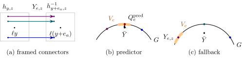
At a step \(m + 1 \to m\), the fine links \(U\) and coarse links \(V\) live on \(\Lambda_{L_p D_{m + 1}}\) and \(\Lambda_{L_p D_m}\); put \(j = J_{m + 1}\), \(\ell = \ell_m\) and \(\mathbb{B}_R = \{- R, \ldots, R\}^4\). Fine transports between two coarse endpoints are compared after expressing them in the same frames. A frame is a gauge transformation \(h_{y, z} \in G\) at each fine site \(\ell y + z\) of the patch of radius \((j + 3) \ell\) around \(\ell y\), built from parallel transports in the patch (Definitions 11.1–11.3). For a coarse edge \(e = (y, a)\) the framed straight connector is
| \(\displaystyle Y_{e, z} = h_{y, z} \left( \prod_{r = 0}^{\ell - 1} U (\ell y + z + re_a, a) \right) h_{y + e_a, z}^{- 1} \hspace{0.17em},\) | (5.4) |
the fine transport from \(\ell y + z\) to \(\ell (y + e_a) + z\) in the frames at its ends. With \(\text{Unif}\) the uniform probability on a box and \(\ast j\) the \(j\)-fold convolution, the averaging weights and the predictor are
The second form holds because \(\text{pr} (Yu^{- 1}) = (2 n_G)^{- 1} \|Y - u\|_{\text{F}}^2\) for unitary \(Y, u\): the predictor is the point of \(G\) nearest to the weighted average of the connectors, an average of group variables taken through the ambient matrices. On a good patch the connectors lie near one another, and this branch, on which the minimizer is unique, is used when the minimum lies below a fixed cutoff. Where the frame test or the predictor test fails, the kernel chooses at random, an axial frame from a finite list or a single connector \(Y_{e, z}\) with probability \(w^{\text{av}}_z\); these branches complete the kernel on the remaining configurations (Section 11 gives the decision rules, summarized in Table 4 and Figure 8). A tag \(\alpha_{\text{tag}}\) records these discrete choices and nothing else: for each coarse site a frame label \((z, o)\), an offset \(z \in \mathbb{B}_{(j + 3) \ell}\) and an order \(o\) of the four axes, and for each coarse edge an offset \(z \in \mathbb{B}_{(j + 3) \ell}\) selecting a connector; on the minimizing branches the label is drawn uniformly and does not affect the kernel. Tags are drawn with probabilities
| \(\displaystyle \lambda^{\text{tag}} (U, \alpha_{\text{tag}}) \geqslant 0, \qquad \sum_{\alpha_{\text{tag}}} \lambda^{\text{tag}} (U, \alpha_{\text{tag}}) = 1 \hspace{0.17em} .\) | (5.6) |
Given \(U\) and the tag, the coarse links are independent, each concentrated within about \((\textsf{b} \beta)^{- 1 / 2}\) of its predictor, with the normalized density \(q_{\gamma} (u) = e^{- \gamma \text{pr} (u)} / \int_G e^{- \gamma \text{pr}} \hspace{0.17em} dh\); the block penalty plays the role of the smearing parameter of soft block-spin transformations.
Definition
with probability Haar measures on both link sets.
For fixed \(U\) and tag, right invariance of Haar measure makes each coarse factor integrate to one; summing the tag masses gives \(\int k^{(m)}_{\beta} (U, V) \hspace{0.17em} dV = 1\). Hence, for integrable \(f\),
| \(\displaystyle \int (\mathcal{B}^{(m)}_{\beta} f) (V) \hspace{0.17em} dV = \int f (U) \hspace{0.17em} dU \hspace{0.17em} :\) | (5.7) |
the map integrates one scale exactly and keeps the partition integral. Branches, measurability and symmetries of the kernel are proved in Section 11.
Probabilistically, a block step is the following experiment. Let \(U\) have law \(f (U) \hspace{0.17em} dU / \int f\) for an integrable \(f \geqslant 0\) with \(\int f > 0\); draw a tag with probabilities \(\lambda^{\text{tag}} (U, \cdot)\); and put \(V_e = R_e Q_e^{\text{pred}} (U, \alpha_{\text{tag}})\), where the \(R_e\) have density \(q_{\textsf{b} \beta}\) and are independent of each other and of \((U, \alpha_{\text{tag}})\). The pair \((U, V)\) then has law \(f (U) k^{(m)}_{\beta} (U, V) \hspace{0.17em} dU \hspace{0.17em} dV / \int f\), and by Fubini the law of \(V\) has density \(\mathcal{B}^{(m)}_{\beta} f / \int f\) with respect to Haar measure. Exactness refers to this identity, which includes every branch of the kernel. It does not mean that the coarse density is again a Wilson density; Section 5.2 gives the coordinates in which it is written.
The density produced by the integrations records four things: the leading curvature action with its running coupling, the field-independent scalar accumulated so far, small local corrections on small-field supports, and the contributions of large-field regions. At level \(m\) write \(\Lambda = \Lambda_{L_p D_m}\). The flagged sites \(\text{Flag}_m (U)\), or large-field sites, are the sites incident to a plaquette whose chord exceeds \(t_m\); a support is healthy, or small-field in the sense of Bałaban, if it contains none. Flags are gauge invariant, because plaquette chords are: the transform of the identity configuration in Section 2.1 has no flagged site, however far its links are from the identity. A regular activity \(E_i^{\text{reg}}\) is a Borel real gauge-invariant function, local on its support \(X_i\), anchored at \(o_i \in X_i\) and vanishing at the flat configuration; it is used only on healthy supports. A forced activity \(K_i^{\text{for}}\), one of the large-field polymer activities, is local on its support \(Y_i\) and carries a nonempty inventory \(I_i \subset Y_i\) of flagged sites; it vanishes off its eligibility event
The first condition fixes exactly which sites of \(Y_i\) are flagged. The extra event is a fixed Borel gauge-invariant test supplied with the activity, which reads only links with both endpoints in \(Y_i\) and the flags in \(Y_i\); it distinguishes local alternatives with the same support and inventory. The activity families are countable.
The path action carries the kinetic coefficient and the quadratic corrections generated by integration. At level \(m\) abbreviate the clipping constants and relaxation length of item 4 of Table 3,
where \(\gamma_j > 0\) is half a uniform lower bound for the free effective plaquette forms of Lemma 11.5. Distances are periodic maximum-coordinate distances in lattice units: on a torus of side \(n\), \(\text{dist} (x, y) = \min_{z \in n\mathbb{Z}^4} | \tilde{x} - \tilde{y} + z|_{\infty}\) for lifts \(\tilde{x}, \tilde{y} \in \mathbb{Z}^4\). Set
For each plaquette orientation \(\mathfrak{p}= (a, b)\), let
\(\mathcal{F}_{\mathfrak{p}i} (U, x)\) be a curvature
\(\text{proj}_{\mathfrak{g}} (U_{\square} - U_{\square}^{- 1}) / 2\),
with the orthogonal projection for the metric of Definition 2.1,
transported along a specified finite path to \(x\), and put
\(\mathcal{L}_{\mathfrak{p}}^{\text{path}} (U, x) = \sum_i
r_{\mathfrak{p}i}
\mathcal{F}_{\mathfrak{p}i} (U, x)\), a smeared
lattice curvature at \(x\). The action splits the effective kinetic form
into a clipped part, quadratic below \(t_m\) and linear beyond, and the
remaining positive form, written as a sum of squares with one row per
\((x, \mathfrak{p})\); a row is switched off once some plaquette exceeds
its distance-relaxed threshold, that is, when the relaxed threshold
test \(\chi^{\text{rel}}_{m, x}\) of
where \(h^{\ast} U\) transports links by the lattice isometry \(h\). The path coefficients and multilinear expressions are independent of \(p\) (Definitions 12.1–12.2, Lemmas 12.3–12.4); the action is affine in \(\beta\),
where, after the average over \(H_4\), \(\partial_{\beta} P^{\text{path}}_{N, m}\) collects the clipped plaquette terms, the row squares with their switches \(\chi^{\text{rel}}_{m, x}\) and the cubic and quartic terms, and \(P^{\text{path}}_{N, m} (0, \cdot)\) the quadratic terms \(\mathfrak{a}_i^{(2)}\). The clip drops at \(r = t\) from \(c_{\text{dir}} t^2 / 2\) to \(c_{\text{lin}} t^2\). Accordingly the density coordinates are Borel functions; derivatives are taken only on healthy configurations with the masks held fixed, so coupling derivatives never differentiate the flag boundary. The positive linear branch beyond the threshold is what the local large-field energy bound (Lemma 11.12) uses.
For these fixed path actions and thresholds, a representation at level \(m\) is the datum
| \(\displaystyle \rho = (\beta, v_{\text{sc}}, (X_i, o_i, E_i^{\text{reg}})_i, (Y_i, I_i, \mathcal{E}_i^{\text{extra}}, K_i^{\text{for}})_i) \hspace{0.17em},\) | (5.11) |
with scalar normalization per site \(v_{\text{sc}}\) (a constant in the effective density, not the vacuum vector of Section 6.3) and running coupling \(\beta (\rho) = \beta\). The running coupling is thus a coordinate fixed by the choice of path action: the coefficient of the fixed function \(\partial_{\beta} P^{\text{path}}_{N, m}\), whose quadratic part is normalized so that \(\beta\) is the coefficient of the squared curvature at zero momentum at every level, while the quadratic terms \(\mathfrak{a}_i^{(2)}\) carry no curvature-square term (Lemma 12.4). It is not read off from the whole density, which also contains \(v_{\text{sc}}\) and the activities. Let \(\mathfrak{F}_m (U)\) be the set of finite \(\mathfrak{a} \subset \mathbb{N}\) such that the supports \(Y_i\), \(i \in \mathfrak{a}\), are pairwise disjoint and \(\bigcup_{i \in \mathfrak{a}} I_i = \text{Flag}_m (U)\): the exact covers of the flagged sites.
Definition
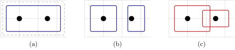
If there are no flagged sites, \(\mathfrak{F}_m (U) = \{\varnothing\}\) and the forced sum is one. Otherwise every flagged site lies in exactly one selected support, but the sum runs over all exact covers: one support may carry two flags in one term while two disjoint supports carry one flag each in another (Figure 4). The local regularity of the activities and the restrictions on forced terms are Definitions 13.1–13.2.
|
Figure 4. Exact covers of two flagged sites (dots). (a) One support carries both flags; the dashed line marks the larger region its eligibility test inspects. (b) Two disjoint supports carry one flag each. Both selections occur in the sum of Definition 5.2, which does not choose a canonical cover. (c) Overlapping supports are not a cover. |
For a link \(e\) let \(e^-\) be its initial site. The left derivative \(D^L_{\dot{\mathcal{A}}}\) differentiates the increments \(U_e \mapsto e^{t \dot{\mathcal{A}}_e} U_e\), with \(\dot{\mathcal{A}}_e \in \mathfrak{g}\) normed by Definition 2.1.
Definition
over configurations healthy on \(X_i\) and directions with \(| (\dot{\mathcal{A}}_k)_e | \leqslant t_m (1 + \text{dist} (e^-, o_i))^{\varpi_{J_m}}\), \(1 \leqslant k \leqslant q\).
The seminorm measures ordered local derivatives in units of the permitted field size. For a support \(X\), let \(\text{cov}_{B_m} (X)\) be the least number of radius-\(B_m\) lattice balls with connected union covering \(X\); the exponential weight below penalizes supports that need many such balls.
Definition
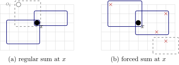
The two sums are formed differently (Figure 5). The regular sum at \(x\) counts the activities anchored at \(x\), whatever their supports, so each regular activity is counted once, at the site from which its derivative directions are weighted (Definition 5.3). The forced sum at \(x\) counts every forced activity whose support contains \(x\), so the weight \(e^{\sigma_{J_m} \text{cov}_{B_m} (Y_i)}\) charges a large support at each of its sites; if \(x\) is flagged, every activity that covers \(x\) in a term of Definition 5.2 is counted there. Section 13 converts anchored bounds into containing-site bounds where needed, at the cost of the number of possible anchors of a support.
|
Figure 5. The weighted sums of Definition 5.4 at a site \(x\). (a) The regular sum counts the activities anchored at \(x\) (solid supports), whatever their extent; the dashed support contains \(x\) but is anchored at \(o_i \ne x\) and is counted at \(o_i\). (b) The forced sum counts every activity whose support contains \(x\) (solid), whatever its inventory (crosses); overlapping supports both count, since the sum runs over activities, not covers. The dashed support does not contain \(x\). |
The induction keeps the bounds
| \(\displaystyle \mathcal{E}_m \leqslant \epsilon_m^{\text{reg}}, \qquad \mathcal{K}_m \leqslant \epsilon_m^{\text{for}} \hspace{0.17em} .\) | (5.12) |
These numerical bounds do not by themselves define the classes on which the step acts. The Wilson start is the continuous curve
with scalar normalization zero (Lemma 13.16). The
admissible classes consist of everything reachable from it. Let
\(\mathcal{I}_{N, p} = \{\rho^{\text{W}}_{\beta} : \beta \in
\mathfrak{B}_N \}\) and \(\mathcal{A}_{N, N, p} =\mathcal{I}_{N, p}\).
For \(m < N\), a representation at level \(m\) belongs to
\(\mathcal{A}_{N, m, p}\) if it is obtained from some \(\rho' \in
\mathcal{A}_{N, m + 1, p}\) with coupling in \(\mathfrak{B}_{m + 1}\) by
one block step of Section 13: its path is
\(P^{\text{path}}_{N, m}\), its activities are produced by local
subtraction, path replacement and fusion, its coupling is that of
\(\rho'\) plus the one-loop coefficient \(\alpha_{N, m}\) of Lemma 12.9 and a correction bounded by the first inequality of
Exact integration removes one scale. Extracting its marginal curvature-square term into the coupling leaves a bounded drift error and returns a density in the next admissible class.
Theorem
Idea of the proof (Sections 11–13; the proof follows Lemma 13.17).
The density identity is exact because the output coordinates rewrite
the block-integrated density on every configuration (Lemma 13.13);
by
On small fields, gauge fixing in a rooted block-tree gauge and the stationary background turn the local integral into a Gaussian integral with its determinant and Haar-coordinate factors; the large-field lower bound (Lemma 11.12) pays for the forced terms.
Classical fourth-order matching fixes the local terms, and the background curvature-square coefficient of the one-loop action, assembled from the inherited quadratic loop term, the fluctuation determinant and the Haar Jacobian, gives the change \(- \kappa_G \log \ell_m\) up to a stage-bounded error (Lemma 12.9).
The local expansion, the contraction of inherited terms and the five-torus localization (Lemma 4.1) give the regular bound; forced fusion gives the forced bound; the scalar coupling reset absorbs the residual kinetic coefficient (Lemma 13.14).
The bound \(\omega_j^{\text{RG}}\) depends only on the stage, not on \(N, p\), the interval or the curve. Since \(\hat{\beta}_m = \hat{\beta}_{m + 1} - \kappa_G \log \ell_m\), a step changes \(\beta - \hat{\beta}\) by \(e_u\) only.
A trajectory is a tuple \(\rho_{N, p, m} \in \mathcal{A}_{N, m, p}\), \(0 \leqslant m \leqslant N\), with \(\rho_{N, p, N} \in \mathcal{I}_{N, p}\) and \((\rho_{N, p, m}, \rho_{N, p, m + 1}) \in \mathcal{R}_{N, m, p}\) for \(m < N\); write \(\beta_{N, p, m} = \beta (\rho_{N, p, m})\). The bare coupling is selected by shooting. Put \(\mathfrak{T}_m = [\bar{\beta} + \tfrac{\kappa_G}{2} s_m, \bar{\beta} + 2 \kappa_G s_m] \subset \mathfrak{B}_m\), so that \(\mathfrak{T}_0 = \{ \bar{\beta} \}\). Start with the Wilson curve on \(\mathfrak{T}_N\). Suppose a closed parameter interval has level-\((m + 1)\) couplings in \(\mathfrak{T}_{m + 1}\), taking its end values at its endpoints. Since \(s_{m + 1} = s_m + \log \ell_m\) and \(|e_u | \leqslant \omega^{\text{RG}}_{J_{m + 1}} \leqslant \tfrac{\kappa_G}{4} \log \ell_m\) (item 5 of Table 3), the output couplings at the two endpoints satisfy
The intermediate value theorem gives a closed subinterval whose couplings lie in \(\mathfrak{T}_m\) and take its end values at its endpoints. After \(N\) steps the level-zero coupling is \(\bar{\beta}\). The couplings are chosen this way for all \(N, p\) before any sequence of volume indices is prescribed. Trajectories for different cutoffs thus share the coupling \(\bar{\beta}\) at level zero; their scalar normalizations and activities need not agree (Figure 6), and Proposition 5.7 below compares them at a fixed level as the cutoff grows.

|
Figure 6. Trajectories for two cutoffs \(N < N'\) at one volume, from the Wilson start at the cutoff (left) to level zero (right); each arrow is a block step, and levels are aligned vertically. Both reach the coupling \(\bar{\beta}\) at level zero; their scalar normalizations and activities need not agree. At a fixed level \(m\) (dashed), Proposition 5.7 gives convergence of the couplings and activities as the cutoff tends to infinity. |
Theorem
For every \(\varepsilon > 0\), some \(m_0 (\varepsilon)\) satisfies
The proof is the shooting argument above (Section 14.1,
Lemmas 14.2–14.3). Fix these
trajectories for all later constructions. The drift bound of Theorem 5.5 holds on every adjacent pair, and all their integrals
equal \(Z_{L_p D_N, \beta_{N, p}}\) by
| \(\displaystyle | \beta_{N, p, m} - \hat{\beta}_m | \leqslant \sum_{i = 0}^{m - 1} \omega_{J_{i + 1}}^{\text{RG}} \hspace{0.17em} .\) | (5.14) |
Item 5 of Table 3 bounds the sum by \((\kappa_G / 4) s_m\), which also keeps the couplings in \(\mathfrak{B}_m\). Its stronger bound \(\omega_{J_{i + 1}}^{\text{RG}} \leqslant J_{i + 1}^{- 2} \log \ell_i\) makes the sum \(o (s_m)\): split it at a fixed level and bound the tail by \(\sup_{i \geqslant i_0} J_{i + 1}^{- 2}\) times \(s_m\). Since \(J_i \to \infty\) and \(s_m \to \infty\), the finite initial sum and \(\bar{\beta}\) disappear after division by \(s_m\), uniformly in \(N \geqslant m\) and \(p\). As \(\omega_j^{\text{RG}} \geqslant 1\), the same bound forces \(\log \ell_m \geqslant J_{m + 1}^2 \to \infty\): the block ratios must grow, and the level choices also give \(\log \ell_m / s_m \to 0\). The step construction of Theorem 5.5 is fixed once on whole continuous curves (Lemma 13.17); the trajectories it produces from \(\rho^{\text{W}}_{\beta}\), and their restrictions, form the specified recursion, to which the trajectories of Theorem 5.6 belong. Different cutoffs are compared through the following limit.
Proposition
Idea of the proof (Lemmas 13.22 and 13.24). The argument uses geometric truncation, not compactness of a ball in an infinite-dimensional space. The scalar coordinates lie in fixed compact intervals, so a diagonal argument gives subsequential limits. At a fixed higher level \(k\), replace the activity coordinate by zero and run the same maps down to level \(m\): the error is at most \((8 g_{\ast})^{k - m}\) with \(g_{\ast} = 1 / 128\), uniformly in the cutoff, while the truncated coordinates converge by the cutoff compatibility of finitely many step maps (Lemma 13.22). Letting \(k \to \infty\) gives the activity limits. Two limits have the same endpoint \(\bar{\beta}\), and their distance \(\mathfrak{d}_{\infty}\) satisfies \(\mathfrak{d}_{\infty} \leqslant 8 g_{\ast} \mathfrak{d}_{\infty}\), so they coincide.
Blocking a density that carries one insertion returns a density of the same form: the unmarked density times a local insertion with new coefficients, plus regular remainders with vanishing Taylor coefficients through order \(d\) and forced remainders attached to large fields. The coefficients evolve linearly, and the insertions of Definition 2.8 are normalized by prescribing them at the reference level. Choose the reference level \(m_{\text{ref}} (d)\) with \(J_{m_{\text{ref}} (d)} \geqslant d + 3\) and \(\mathfrak{q}_{J_m} \geqslant d + 1\), \(\varpi_{J_m} \geqslant d\) for \(m \geqslant m_{\text{ref}} (d)\) (Lemma 14.7). Fix \(N \geqslant m_{\text{ref}} (d)\); starting from a fine-cutoff coefficient vector \(\mathbf{v} \in V_d\), the marked density at the origin is initialized and blocked by
For fixed \(N, p, d\), the transfer construction chooses coefficient vectors \(\mathbf{x}_m (\mathbf{v})\) and regular and forced remainders \(R_{m, i}^{\text{reg}} (\mathbf{v})\), \(Q_{m, i}^{\text{for}} (\mathbf{v})\), all linear in \(\mathbf{v}\). Write \(\mathbf{x}_m = x_{m, 0} \boldsymbol{1}+\mathbf{x}_m^{\circ}\) and \(\rho_m = \rho_{N, p, m}\). The regular remainders have supports \(Z_{m, i}\) containing the origin. Their sum and the forced remainder are
with all unmarked quantities taken from \(\rho_m\). The marked density has the exact decomposition
with the stencil \(\Sigma_d\) placed at the origin of the level-\(m\) torus. If \(10 \text{dist} (x, 0) < L_p D_m\) for every \(x \in Z_{m, i}\), the regular remainder \(R_{m, i}^{\text{reg}}\) has zero radial-jet Taylor coefficients through order \(d\); the forced remainders vanish outside their unmarked eligibility events (Lemmas 14.7–14.9). The fixed decomposition selected there gives the terminal map of Definition 2.8, invertible by Lemma 14.7:
The factor \(\ell_m^d = (a_m / a_{m + 1})^d\) uses the degree of the whole space \(V_d\), and the terminal map accounts for the mixing between its weights. The unit identity \(\mathbf{x}_m (a_N^d \boldsymbol{1}) = a_m^d \boldsymbol{1}\), proved with the transfer symmetries (Lemma 14.8), explains why the coefficient of the constant insertion is \(a_{m_{\text{ref}} (d)}^d \boldsymbol{1}\), although \(V_d\) also contains polynomials of lower weight. With Theorem 5.6, these insertions specify one Wilson family; each insertion is continuous, gauge invariant and local on its fixed stencil, and Theorem 5.6 at \(m = N\) gives the volume-uniform slope \(\kappa_G > 0\).
For a finite list \(\boldsymbol{l}\) of pairs \((i, a)\), with \(i\) a slot and \(a\) an axis, the normalized differences and derivatives are
where \(\tau_{i, a}\) shifts slot \(i\) forward by one lattice link. The torus separation of a lattice tuple is \(\min_{i \ne j} \min_{z \in L_p \mathbb{Z}^4} | \hat{y}_i - \hat{y}_j + z|_{\infty}\), with value \(+ \infty\) for \(n \leqslant 1\), and
the last set excludes collisions on a torus of physical side \(L\). The first result bounds lattice correlations and their differences independently of the volume.
Proposition
Idea of the proof (Section 14.2). Choose an
intermediate level whose physical blocks fit below the separation, so
the insertions lie in distinct blocks. By the decomposition
for \(O_i\) localized in distinct blocks and \(\mathcal{G}\) generated by the reflections in the block boundaries; each factor is independent of the volume. The reflected-moment constant is chosen before the intermediate level, and only the cutoff threshold depends on it.
The second result removes the spacing at each fixed volume along the full sequence; Section 4.2 displays the Cauchy argument.
Theorem
Idea of the proof (Lemmas 14.33–14.34). The Cauchy argument of Section 4.2 gives convergence on \(\bigcup_m a_m \mathbb{Z}^4\): the transferred correlations at a fixed level converge, and the stopping error \(2 F_0 e^{- B_m / 64}\), with \(F_0\) independent of \(m\), compares them with the original ones. Proposition 5.8 extends convergence to all separated positions and identifies every derivative, also at moving points crossing the boundary of the chosen period cell. For \(\boldsymbol{l}= \varnothing\) the left side is \(\lim_N C^{\text{lat}}_{N, p} (v ; f)\), so the inner limits of Definition 2.6 exist at every admissible volume; admissibility places the support of \(f\) inside \(\text{NoHit}_{L_p, n}\). The limiting kernel is periodic in each position and smooth away from periodic collisions, including where positions share coordinates. The thresholds may depend on \(p\).
The lattice family of Section 5 is now fixed; its couplings and insertions were chosen before any sequence of volume indices. This section takes the volume limit and identifies the continuum fields: their calculus, the stress tensor and the rotations, the phases and their reconstruction, the trace law and the products. Constants may depend on the group, its realization, the penalty and the construction choices of Section 9; further dependence is stated.
One volume refinement serves every field and all later constructions.
Theorem
Remark
Fix \(\textsf{p}\), \(\textsf{q}\), \(P\) and \(S\) from now on.
Idea of the proof (Lemmas 15.1–15.6).
Proposition 5.8 bounds the correlations and all their lattice differences uniformly in the volume; a diagonal extraction along \(\textsf{p}\) gives local smooth limits on \(\text{Conf}_n\) (E6). At each admissible volume the fixed-volume kernels are those of Theorem 5.9, so the full inner limit is kept; only the outer limit uses a subsequence.
The chessboard seminorm, the cost of repeating one observation throughout the box, gives E7 at order zero, and the corrected derivative maps below give it at positive orders; lattice reflection positivity passes to the limit, giving E5 and then E4.
A further refinement fixes finitely many coefficient maps in each degree. This auxiliary subsequence concerns finite-dimensional coefficients only; the limits of the correlations are the full ultraviolet limits already established.
The coefficient maps are needed because the normalization \(a_N^{- d} \textsf{Z}_{N, p, d}^{- 1}\) depends on the degree. The same \(c \in V_d \subset V_e\) defines different lattice fields as \((d, c)\) and as \((e, c)\), and a lattice difference of a degree-\(d\) insertion is a degree-\((d + 1)\) object with yet another normalization; the naive inclusion \(V_d \to V_e\) does not preserve correlations. Lemma 15.5 constructs linear corrected coefficient maps relating these normalizations, and they induce the inclusions and derivatives of the next proposition. Its dimension statement uses a Gaussian comparison theory, introduced by its covariance.
Definition
the derivatives taken in the sense of distributions. Let \(M_d^{\text{Max}}\) consist of the complex \(\text{Ad} (G)\)-invariant Wick polynomials in curvature jets of weight at most \(d\), modulo antisymmetry, the linear Bianchi identities and \(\sum_a \partial_a F_{ab} = 0\). Their separated Wick correlations are \(S^{\text{Max}}\).
Each component of \(A\) is a massless free field, with covariance \((- \Delta)^{- 1}\) since \(- \Delta \Gamma = \delta_0\), and \(F\) is the free Maxwell field. Wick polynomials in curvature jets at distinct points have smooth correlations, computed by Wick's theorem from derivatives of \(\Gamma\) at nonzero arguments. The relations are of two kinds. Antisymmetry and the Bianchi identities \(\partial_a F_{bc} + \partial_b F_{ca} + \partial_c F_{ab} = 0\) hold identically, since \(F\) is a derivative of \(A\). The equation \(\sum_a \partial_a F_{ab} = 0\) holds only in separated correlations: by \(- \Delta \Gamma = \delta_0\),
which vanishes for \(x \ne y\), so every separated Wick correlation with a factor of the divergence vanishes; but the divergence is not the zero distribution, since its covariance is \(\delta_{\alpha \beta} (\partial_b \partial_d - \delta_{bd} \Delta) \delta_0 (x - y)\). The quotient by this equation thus records a relation among separated correlations, not an identity of distributions. The comparison of Proposition 6.7 likewise concerns separated correlations at short distances; it does not identify the constructed fields with this Gaussian reference.
The constant one is the Maxwell unit, coefficient conjugation gives the real structure, and inclusions keep the same polynomial at a larger weight bound. Free differentiation is \(\partial_a^{\text{Max}} (: P :) = : \partial_a P\):, and the rotation action \(R_d^{\text{Max}} (h) (: P :) = : hP\): is determined by \(hF_{ab}^{\alpha} = \sum_{i, j} h_{ia} h_{jb} F_{ij}^{\alpha}\) and \(h \partial_a = \sum_i h_{ia} \partial_i h\) for \(h \in O (4)\); these operations preserve the defining relations.
Proposition
The proof is Lemma 15.5. The corrected coefficient maps supply representatives of inclusions and derivatives; the equation and rank comparisons of Lemmas 14.18–14.26 bound \(\dim F_d\) from above, and the free tests of Lemma 14.22, with the free positivity of Lemma 16.1, bound it from below. Each \(\iota_d\) is injective by Definition 2.12, so the inclusions are unique and injective, \(\jmath_{e, f} \jmath_{d, e} = \jmath_{d, f}\), \(\jmath_{d, d} = \text{id}\), and by E1 they carry \(\boldsymbol{1}_d\) to \(\boldsymbol{1}_e\). Their images are nested, so \(\mathcal{L}= \bigcup_d \iota_d F_d\). Permutation symmetry gives, for \(\boldsymbol{A} \in \prod_i F_{d_i}\), \(x \in \text{Conf}_n\), slot \(i\) and axis \(a\),
and E2 with injectivity of the responses makes inclusions and derivatives commute with conjugation, inclusions commute with \(H_4\), and \(h \partial_a = \sum_b h_{ba} \partial_b h\) for \(h \in H_4\).
The table also defines reflection Hilbert spaces along the coordinate axes. They and their slab bounds use only the volume limit and the field calculus (Lemmas 15.6, 15.7 and Proposition 6.4), and they enter the rotation argument of Section 6.2 before continuous rotations are available.
Definition
By E4 the form is positive semidefinite; with E7, the translations \(\tau_{te_a}\), \(t \geqslant 0\), preserve its null space and define a strongly continuous self-adjoint contraction semigroup, whose generator is \(H_a^{\text{OS}} \geqslant 0\) (proof of Lemma 16.12). Inserting a word between positive-time vectors is bounded after a positive time translation (Lemma 16.12); these slab bounds are the coordinate estimates used before rotations.
The fields are compared with Maxwell fields at small distances, through bases that may vary with the radius to accommodate mixing, and a conserved tensor is then normalized by its shell fluxes. The volume refinement and \(S\) remain fixed; the subsequences below concern comparison radii only.
Definition
After rescaling positions the interacting correlations approach their Maxwell counterparts; one sequence serves every fixed list of fields.
Proposition
Idea of the proof (Lemma 16.8). The lattice comparison stops near the requested physical scale and compares the correlations with the free Gaussian ones. Finitely many separating correlations make the comparison maps injective, the upper bound \(\dim_{\mathbb{C}} F_d \leqslant \dim_{\mathbb{C}} M_d^{\text{Max}}\) of Proposition 6.4 makes them isomorphisms, and finite-dimensional corrections impose the eventual equalities. Local \(L^1\) convergence is equivalent, by duality and smooth approximation on slightly larger separated compact sets, to convergence uniform over smooth tests with \(\|f\|_{\infty} \leqslant 1\) and fixed compact support. This weaker form is used to construct and normalize the conserved current, before the stress tensor exists.
To read translation and angular charge, integrate a conserved symmetric tensor through a shell surrounding one insertion. In a free model the shell integral can be computed, and it differentiates the enclosed correlation. Let \(\phi\) be a massless free scalar field with covariance \(\Gamma\), write \(\langle \cdot \rangle\) for its Wick correlations, and put \(T^{\phi}_{ab} = - : \partial_a \phi \hspace{0.17em} \partial_b \phi : + \frac{1}{2} \delta_{ab} : | \nabla \phi |^2\):, the negative of the canonical tensor. With \(\Gamma_0 = \Gamma (y - x_0)\) and \(\Gamma_1 = \Gamma (y - x)\),
whose divergence in \(y\) vanishes away from \(x_0\) and \(x\), where \(\Delta \Gamma_0 = \Delta \Gamma_1 = 0\). Take a smooth compactly supported \(\chi\) equal to one on the ball of radius \(\epsilon < |x - x_0 |\) about \(x_0\) and vanishing near \(x\). The divergence theorem turns the flux \(- \sum_a \int \partial_a \chi (y) \langle T^{\phi}_{ab} (y) \phi (x_0) \phi (x) \rangle \hspace{0.17em} dy\) into the integral of \(\sum_a \langle T^{\phi}_{ab} (y) \phi (x_0) \phi (x) \rangle n_a\) over the boundary sphere of that ball, with outer normal \(n\). There \(\nabla \Gamma_0 = - n / (2 \pi^2 \epsilon^3)\), the last two terms cancel, and the integrand is \(\partial_b \Gamma_1 / (2 \pi^2 \epsilon^3)\). The sphere has area \(2 \pi^2 \epsilon^3\) and \(\partial_b \Gamma (\cdot - x)\) is harmonic on the ball, so the mean value property gives the flux \(\partial_b \Gamma (x_0 - x) = \partial_{x_0^b} \langle \phi (x_0) \phi (x) \rangle\). This free calculation illustrates the identity that Theorem 6.10 establishes for the constructed fields by a different route.
We normalize the stress tensor in the same way, so that its translation flux acts as \(+ \partial_{x_0^b}\) on the enclosed insertion; with the minus sign in the flux below, this gives the negative of the usual Euclidean canonical Maxwell tensor (displayed after Theorem 6.10). Let \(A \in F_d\), let \(\boldsymbol{B}\) be a list of \(n\) spectator fields at \(x\), and take \((x_0, x) \in \text{Conf}_{n + 1}\).
Definition
The integrals avoid every insertion point, and they do not depend on the shell cutoff: two choices differ by a function vanishing near every insertion, integration by parts with Proposition 6.4 removes the divergence term, and the extra angular term is \(\sum_{a, b} (K_{\text{rot}})_{ba} J_{ab} = 0\) since \(K_{\text{rot}}\) is skew and \(J\) symmetric. Conservation makes the flux independent of the radius of the shell; it does not by itself control a flux through a distant surface. A field is real when fixed by conjugation; a family \(J_{ab} \in F_4\) is \(H_4\)-tensorial when \(hJ_{ab} = \sum_{i, j} h_{ia} h_{jb} J_{ij}\) for \(h \in H_4\), conserved when \(\sum_a \partial_a J_{ab} = 0\) in \(F_5\) for every \(b\), and centered when every component has zero one-point function.
Proposition
This is the first assertion of Lemma 16.10; its proof shows that divergence maps the centered real symmetric tensorial families onto the corresponding vectors in degree five, with one-dimensional kernel. Along a refinement of the sequence of Proposition 6.7, positive multiples of the rescaled nonzero member approach the free stress line in the degree-four frames. For a nonzero member \(J\), Lemma 16.11 constructs complex linear charge maps \(\textsf{p}_b : F_d \to F_{d + 1}\) and \(\textsf{Y}_{K_{\text{rot}}} : F_d \to F_d\), the latter real linear in \(K_{\text{rot}}\), with \(\mathcal{P}_b^J = S ((\textsf{p}_b A) (x_0), \boldsymbol{B}(x))\) and \(\mathcal{Y}_{K_{\text{rot}}}^J = S ((\textsf{Y}_{K_{\text{rot}}} A) (x_0), \boldsymbol{B}(x))\) for every degree, field, spectator list, separated configuration and shell cutoff.
These charges restore the rotations. Conservation of \(J\) turns the sum of the angular charges of the insertions, each combining \(\textsf{Y}_{K_{\text{rot}}}\) at its own point with the translation charge weighted by the rotated position, into the integral of \(J\) against the derivative of a vector field equal to \(y \mapsto K_{\text{rot}} y\) on a large anisotropic box. For configurations on a coordinate line, the coordinate reflection spaces of Definition 6.5 show that this integral tends to zero as the box grows (Lemma 16.15; Section 4.3 explains the mechanism), so the angular sum vanishes there. Finite Ward tests then identify \(\textsf{p}_b\) with \(c_{\star} \partial_b\), and analyticity extends the identity, infinitesimal rotation invariance, to all separated configurations. Lemma 16.17 thereby constructs continuous complex linear representations \(R_d\) of \(O (4)\), extending \(H_4\), fixing units and commuting with conjugation and inclusions; for a real \(c_{\star} \ne 0\) common to every degree,
Integrating gives full covariance (Lemma 16.17): \(S_n (R_{d_i} (h) A_i ; hx) = S_n (\boldsymbol{A}; x)\) for every \(\boldsymbol{A} \in \prod_i F_{d_i}\), \(x \in \text{Conf}_n\) and \(h \in O (4)\). A family is \(O (4)\)-tensorial if \(R_4 (h) J_{ab} = \sum_{i, j} h_{ia} h_{jb} J_{ij}\) for every \(h \in O (4)\). The common constant \(c_{\star}\) fixes the normalization of the stress tensor by its action on fields.
Theorem
The proof is in Lemmas 16.17–16.18: divide \(J\) by \(c_{\star}\) and average its tensor transform over \(O (4)\) with probability Haar measure. Covariance and the transformation laws of derivatives and generators give the same shell Ward identities for each transformed current, and integration preserves them, as well as symmetry, reality, centering and conservation. Fix this tensor; it is centered, since \(J\) is and \(R_4\) preserves zero one-point values. The free stress \(T^{\text{Max}}\) is normalized by the same shell Ward identities, with \(\partial_a^{\text{Max}}\) and the free generators \(\textsf{L}_d^{\text{Max}}\) (Section 16.1):
The last comparison includes stress insertions. For a free list \(u_1, \ldots, u_n\), \(u_i \in M_{d_i}^{\text{Max}}\), a stress-slot choice is a subset \(I \subset \{1, \ldots, n\}\) with component pairs \((a_i, b_i)\) for \(i \in I\); put \(A_i^0 = T^{\text{Max}}_{a_i b_i}\) for \(i \in I\) and \(A_i^0 = u_i\) otherwise. The shell Ward identities fix the stress normalization, so its comparison insertion needs only the engineering factor \(r_k^4\). Below, \(D_x^j\) differentiates the whole function \(x \mapsto S_n (\boldsymbol{A}_k ; r_k x)\).
Proposition
Fix this refined sequence \((r_k, \textsf{U}_{k, d}^{\text{sc}})\) from now on. The proof follows Lemma 16.19; with \(I = \varnothing\) and \(j = 0\) it gives Proposition 6.7 in uniform form, but the earlier comparison is needed first, to construct the tensor. Along this sequence, for fixed \(d, a, K_{\text{rot}}\), the transported infinitesimal actions converge in operator norm: \(r_k (\textsf{U}_{k, d + 1}^{\text{sc}})^{- 1} \partial_a \textsf{U}_{k, d}^{\text{sc}} \to \partial_a^{\text{Max}}\) and \((\textsf{U}_{k, d}^{\text{sc}})^{- 1} \textsf{L}_d (K_{\text{rot}}) \textsf{U}_{k, d}^{\text{sc}} \to \textsf{L}_d^{\text{Max}} (K_{\text{rot}})\).
Compression to zero energy separates the mixed correlations into phases. In the reflection space of the time axis, a long empty time interval removes the positive-energy components; the word insertions that survive commute on the zero-energy space, and a character of the algebra they generate assigns compatible scalar values to all of them. The phases are these characters. We now use the fourth coordinate as time.
Definition
The slab insertion places \(w\) in the slab \((0, h_{\text{sl}})\) below the translated state. A separated word is translated into a slab to define its compression; Lemma 17.1 proves independence of width and placement and that the compressed operators generate a separable commutative unital C\(\ast\)-algebra
with cyclic and separating vector \(\Omega_4^{\text{OS}}\). Its vacuum state \(a \mapsto \langle \Omega_4^{\text{OS}}, a \Omega_4^{\text{OS}} \rangle\) satisfies \(S (w) = \langle \Omega_4^{\text{OS}}, M^0 (w) \Omega_4^{\text{OS}} \rangle\) by translation invariance; the measure below represents this state on the character space, and the separating property gives full support. Call a character \(\xi\) a phase and \(S^{\xi}\) its table.
Theorem
Each phase satisfies E1–E7 and has exactly the null spaces \(\mathcal{N}_d (S^{\xi}) =\mathcal{N}_d (S)\). The identities of FC, \(O (4)\) covariance and ST hold with \(S^{\xi}\) in place of \(S\), for the same maps and tensor \(T\). For fixed \(w\), \(\xi \mapsto S^{\xi} (w)\) is continuous.
Idea of the proof (Lemmas 16.12, 17.1 and 17.3). The matrix element \(\langle [u], M^0 (w_1) M^0 (w_2) [v] \rangle\) is a limit of correlations of four words placed far apart in time; the long time intervals project onto \(\ker H_4^{\text{OS}}\). The same four words can instead be spread along a second positive coordinate direction, so that the two middle words occur in the opposite order. By \(O (4)\) covariance (Lemma 16.17) both arrangements have the same limit, so \(M^0 (w_1) M^0 (w_2) = M^0 (w_2) M^0 (w_1)\): rotation covariance is an input to the phase decomposition. Reflection positivity holds in each phase because the compressed reflected Gram matrices are positive operators and characters are positive; that no field becomes null in a phase uses the free tests at short distances. Commutativity alone gives neither.
For each phase apply Definitions 6.5 and 6.12 to \(S^{\xi}\), obtaining \(\mathcal{H}_{4, \xi}^{\text{OS}}\), \(H_{4, \xi}^{\text{OS}}\) and \(\Omega_{\xi}^{\text{OS}}\). Fix \(\xi_{\ast}\) in the full-measure set with one-dimensional time-axis reflection ground space supplied by Lemma 17.3; Theorem 6.16 extends ground-space uniqueness to every phase. Two further notions enter the reconstruction and the trace law.
Definition
Definition
For the theory at a phase \(\xi\) write \(\mathcal{H}_{\xi}\), \(\mathcal{D}_{\xi}\), \(\Omega_{\xi}\), \(\Phi_{\xi}\), \(\textsf{T}_{\xi}\), and define its energy by \(\textsf{T}_{\xi} (te_4) = e^{itH_{\xi}}\). Its reflection comparison map is the linear isometry \(\textsf{J}_{\xi}^{\text{OS}} : \mathcal{H}_{\xi} \to \mathcal{H}_{4, \xi}^{\text{OS}}\) with \(\textsf{J}_{\xi}^{\text{OS}} \Omega_{\xi} = \Omega_{\xi}^{\text{OS}}\) that sends each product of smeared fields applied to the vacuum to the norm limit of its heat-regularized positive-time reflection vectors as the ordered heights tend to zero (proofs of Lemmas 17.5 and 17.8).
Theorem
Every bounded operator in the weak commutant of its fields is scalar.
Idea of the proof (Lemmas 17.5–17.11). Reflection positivity supplies the Hilbert spaces and the nonnegative energy; the slab bounds supply the growth estimates behind the boundary values; the restored rotations, continued to boosts, supply Lorentz covariance and, with the continuation, locality. The uniform low-energy estimate of Section 4.4, continuity of the vacuum-subtracted heat pairings and full support of \(\nu\) extend vacuum uniqueness from almost every phase to every phase, so the choice of \(\xi_{\ast}\) stays valid. The same lemmas give joint Schwartz distributions, phase averages and stress continuation.
The label maps are common to all phases. The adjoint is induced by time reflection followed by conjugation, \((\iota_d A)^{\ast} = \iota_d (R_d (\textsf{s}_4^{\text{refl}}) \bar{A})\) (Lemma 17.7). The Lorentz label action is the continuation of \(R_d\) [15]: spatial rotations keep their Euclidean action, and for \(i = 1, 2, 3\) the boost along \(e_i\) has generator \(- i \textsf{L}_d (K_{4 i})\), where \(K_{4 i} = e_4 e_i^{\textsf{T}} - e_i e_4^{\textsf{T}}\) generates rotation in the \((e_4, e_i)\) plane. In particular, a real \(O (4)\)-invariant field gives a Hermitian Lorentz scalar label. Retain the theory at \(\xi_{\ast}\) and suppress its subscript in \(\mathcal{H}, \mathcal{D}, \Omega, \Phi\) and the other relativistic data.
Several ultraviolet statements of different strength are proved, and they should not be confused.
Statement
What it asserts
Running (Theorem 5.6)
A volume-uniform leading logarithmic slope of the bare
coupling of the tuned family
Maxwell comparison (Proposition 6.7)
Convergence along a sequence of radii, through
scale-dependent frames that include field renormalization and
mixing; not a perturbative expansion of each composite
correlation
Stress comparison (Proposition 6.11)
The same, with derivatives and with the normalized
stress insertions
Trace law (Theorem 6.18)
A specific asymptotic through all positive radii, in
the selected phase
The trace is centered in the phase already selected.
Definition
The one-point value is position independent, and centering removes the vacuum contribution in the selected phase. Adding a real multiple of \(\delta_{ab} \boldsymbol{1}_4\) to \(T\) preserves its shell Ward identities, the limit in Proposition 6.11 and \(\Theta\). The fixed stress tensor is centered in the mixture; the selected-phase centering subtracts its own one-point value.
Theorem
As \(r \downarrow 0\) through all positive radii,
The amplitude comes from the free scalar curvature square, with \(\alpha = 1, \ldots, d_{\mathfrak{g}}\) indexing an orthonormal colour basis:
At running coupling \(\beta\) the scalar trace coefficient is \(4 d_2 / \beta\), with \(d_2 = - b_0 / 2\), computed from a lattice Ward identity and the conserved line (Section 4.5, Proposition 18.8); since \(\kappa_G = 2 b_0\), its leading value at radius \(r\) is \(4 d_2 / (\kappa_G \log (1 / r)) = - 1 / \log (1 / r)\), and squaring it with the free correlation gives \(A_G\) (Section 4.5). The comparison needs fourth-order information beyond Proposition 6.7, with the rate that the slowly growing coefficients require; its estimates are uniform in the phase, although the theorem is stated at \(\xi_{\ast}\) only.
Idea of the proof (Section 18; Lemmas 18.1, 18.2, 18.3 and 18.7).
Begin with any sequence of positive radii tending to zero.
Adjustable stopping levels give the comparison along a subsequence, at generic configurations, not at the time-axis pair defining \(G_{\Theta}\).
The positive spectral representation below makes \(G_{\Theta}\) real and nonincreasing; the monotone function is \(G_{\Theta}\) itself, not \(r^8 \log^2 (1 / r) G_{\Theta} (r)\).
By \(O (4)\) invariance, generic separations slightly below and slightly above the target radius bound \(G_{\Theta}\) there from both sides.
Every starting sequence thus has a subsequence with the same normalized limit, which gives the limit through all radii.
The same proof identifies centering on the word domain, \(\Phi (\iota_4 \Theta, f) = \Phi (\iota_4 \tau, f) - e_{\text{tr}} (\int f) \text{Id}_{\mathcal{H}}\), and constructs the unique positive tempered spectral measure \(\mu_{\Theta}\), supported in \(\bar{V}_+\), with
where \(\hat{f}_+ (\mathbf{p}) = \int e^{i\mathbf{p} \cdot x} f (x) \hspace{0.17em} dx\). Its Lorentz invariance and high-energy limits are Lemmas 18.2 and 18.9. Finite Wick profiles cannot reproduce the factor \(r^{- 8} \log^{- 2} (1 / r)\).
Proposition
The reason is the form of the expansions (Lemma 18.10). Each mass-shell kernel has an expansion to every finite order in integer powers of \(r\) and nonnegative powers of \(\log r\), so a finite profile is, to bounded error, a finite sum of monomials \(r^a (\log r)^k\) with \(a \in \mathbb{Z}\), \(k \in \mathbb{N}\). Multiplication by \(r^8 \log^2 (1 / r)\) makes the terms with \(a > - 8\) vanish and the leading remaining nonzero term diverge, so a finite limit must be zero; the positive limit of Theorem 6.18 excludes equality on every interval \((0, \delta)\). Lemma 18.12 treats polynomial mass-shell comparisons, and Lemmas 18.15 and 8.10 give Fock countertests with their own comparison classes.
The phase quantifiers differ from statement to statement, and the following table records them.
Statement
Scope
Slab, comparison and low-energy estimates
Uniform in the phase
Vacuum uniqueness in the proof of Theorem 6.13
Almost every phase (an intermediate step)
Reconstruction, Theorem 6.16
Every phase
Trace law, Theorem 6.18
The selected phase \(\xi_{\ast}\); uniform estimates in
its proof do not change this
Product expansion, Theorem 6.20
Every phase and the mixture; degree cutoff and
spectators fixed before the threshold, states and positions after
it
The product expansion is a decoder, stated for the tables \(S^{\zeta}\), \(\zeta \in \textsf{X} \sqcup \{ \text{mix} \}\), on the common quotient fields. For each degree \(j\), finitely many probe words placed away from the origin, with biorthogonal coordinate functionals, distinguish the fields of \(F_j\). Applied to a cluster of fields at positions \(x\) around a centre \(o\), the probes read off the field with the same answers, averaged over \(O (4)\) and conjugation; lower degrees are removed before the next one is read, and the coordinates in the basis \(O_{j, \lambda}\) are the coefficients \(c_{j, \lambda} (\boldsymbol{A}; x, o)\) (Definitions 19.3–19.5). For two fields, \(A (x) B (0) \sim C^{\boldsymbol{1}}_{AB} (x) \boldsymbol{1}+ \sum_{\lambda} C^{\lambda}_{AB} (x) O_{\lambda} (0) + \cdots\) is tested inside every correlation with distant spectators, and the error after degree \(D\) is at most \(r^{D + 1 - d_A - d_B - \varepsilon}\): for small \(D\) it may still be singular, and what improves with \(D\) is its order. The probes, the bases and the coefficients are fixed once from the mixed table, before spectators, state indices and truncations; spectator and state independence hold by construction, and the content of the theorem is the size of the remainder of Definition 2.19. The coefficients depend on this prescription, the table and the probes; they are not a canonical expansion, and the theorem concerns this one coefficient system.
Theorem
For every pair of finite lists \(\boldsymbol{A}, \boldsymbol{B}\), \(M_{\text{geo}} \geqslant 0\), \(\eta, \delta_{\text{sp}}, \varepsilon > 0\) and \(D \in \mathbb{N}\), some \(r_1 > 0\) gives, for \(0 < r < r_1\), such clusters, \(\delta_{\text{sp}}\)-clear spectators and all state indices \(\zeta\),
Idea of the proof (Lemmas 19.6–19.10). The discarded part is bounded in the compression algebra; evaluation at a character or at the vacuum state does not increase the bound, so it holds in every phase and in the mixture. The bound enters through moments (Lemma 17.2): lattice cluster replacement makes a group of insertions minus its matched field, one insertion at the centre, small in chessboard seminorm; the chessboard estimate applied to \(2 n\) widely translated, alternately conjugated copies bounds the \(n\)th vacuum moment of the compressed remainder \(U\), so that \(\int | \xi (U) |^{2 n} \hspace{0.17em} d \nu (\xi) \leqslant B^{2 n}\) for every \(n\), and continuity in \(\xi\) with full support of \(\nu\) gives \(\sup_{\xi} | \xi (U) | \leqslant B\). Lattice estimates at three scales, the resolution of the insertions, the fusion scale and the exterior cell, give the degree count \(D + 1 - |\boldsymbol{A}|_{\deg}\) up to factors \(e^{o (\log (1 / r))}\), which \(r^{- \varepsilon}\) absorbs for small \(r\). The two thresholds have the separate dependencies of the statement. The estimate holds at each finite truncation \(D\); no series in \(D\) is claimed to converge. Lemmas 19.13–19.14 and Remark 19.15 give nested and integrated estimates.
Contact subtractions use the same original fields and correlations, with separate projections that extract fields through finite correlation probes; their clearance is a radius keeping the collapsed cluster separated from these probes, independent of the spectator clearance \(\delta_{\text{sp}}\). A collision forest is a family of subsets of slots, any two disjoint or nested. Since \(S_n^{\zeta}\) satisfies E7, some contact extension exists by the standard extension theorem for kernels of polynomial growth at the diagonals; the content of the next theorem is that the explicit subtraction of normal Taylor jets along collision forests produces one, with the local order bounds of Lemma 19.21.
Theorem
The proof is in Lemmas 19.19–19.21. For two insertions, write the test in the centroid and one relative coordinate; for each contact degree \(w\) below the critical order \(L\) of the pair, subtract the degree-\(w\) contact projection of the pair at the centroid, tested against the Taylor jet of order \(L - 1 - w\) of the test in the relative coordinate, and the subtracted expression gains in each shell; three or more insertions bring partial collisions and nested or disjoint forests. A separated test extended by zero has vanishing normal jets on every collision diagonal, so only the correlation integral remains. For a general test, Lemma 19.20 controls the contact terms and the signed residuals after the child subtractions, and the shell induction of Lemma 19.21 gives a continuous functional; Lemma 19.19 supplies covariant contact projections with real bases. The extension is a later construction from the separated correlations, not a limit of unsubtracted lattice correlations at coincident points; neither uniqueness, positivity nor contact Ward identities are asserted.
The principal results of Sections 5 and 6 concern one lattice family and one volume refinement; the deduction assembles them in the order of their choices.
Proof of Theorem B.
Fix \(G\) and \(\textsf{b} > 0\), and make the common
choices in the order of Section 9. The Wilson start
Fix the local sections, reference levels and terminal maps on these trajectories; Definition 2.8 defines every insertion, also below its reference level. The local sections are polynomials in the links of their fixed stencils, hence continuous and local, and the terminal maps change only their coefficients, which preserves gauge invariance. Theorem 5.6 at \(m = N\) gives the volume-uniform running law with \(b_{\ast} = \kappa_G > 0\). Thus \(\mathcal{W}\) is regular (Definition 2.5).
Theorem 5.9 gives the full fixed-volume limit for every field and difference list, so every admissible separated test has a full inner limit before any volume extraction. This proves (i).
Given a strictly increasing \(\textsf{p}\), Theorem 6.1 chooses \(\textsf{q}\) and \(S\) with ordered convergence along \(P = \textsf{p} \circ \textsf{q}\) and properties E1–E7; the same extraction fixes the corrected coefficient maps. This proves the table part of (ii).
Define \(F_d = V_d /\mathcal{N}_d (S)\) and \(\mathcal{L}\) by Definition 2.12. Proposition 6.4 gives the inclusions and derivatives, with injective response maps whose images cover \(\mathcal{L}\), and Theorem 6.10 gives the conserved tensor, normalized by its shell fluxes, on these fields.
Theorem 6.13 gives \(\textsf{X}, \nu, S^{\xi}\) on these quotient spaces. Choose \(\xi_{\ast}\) in the full-measure set with one-dimensional time-axis reflection ground space (Lemma 17.3). Theorem 6.16 reconstructs every phase with a unique vacuum, which proves (iii); retain the theory and continuation at \(\xi_{\ast}\).
Set \(\pi_{\text{quo}} (d, \mathbf{c}) = (d, [\mathbf{c}])\); representatives make it onto. The unit response is nonzero since its one-point function is one, so faithfulness in Theorem 6.16 gives a nonzero acting field and, with Step 5, the label clauses of Q3. Theorem 6.13 gives its phase clauses, and the reconstruction gives Q2 and Q4. Assign arbitrary values to the quotient mixture and phase correlations on the collision diagonals; this supplies the function domains of Q0 and has no distributional content, unlike the contact extensions constructed in Step 9. Separated tests vanish there, so ordered convergence is unchanged, and representative independence gives \(S_n^{\text{mix}} (\pi_{\text{quo}} v ; x) = S_n (v ; x)\) on \(\text{Conf}_n\). This identifies the lattice limit \(\mathcal{W} \to S^{\text{mix}} \circ \pi_{\text{quo}}\) of (ii).
Center the trace of the fixed tensor in the selected phase by Definition 6.17. Theorem 6.18 gives vacuum centering, the positive amplitude and the full-radius law, and Proposition 6.19 excludes every finite Wick profile; these give Q6 and (iv).
Choose the underlying prescription of Lemma 19.6 once, with its original fields and correlation table. Theorem 6.20 gives Q5 and its error bounds. Theorem 6.21 and Lemmas 19.19–19.21 use the same prescription, with separate contact projections, separating functionals and clearance, to construct real bases of the contact strata and the contact extensions; the contact proof uses the lattice-derived estimates of Lemma 19.9 and the signed transfer of Lemma 19.20. This proves (v) and completes (ii).
\(\Box\)
Remark
Remark
| \(\displaystyle b_{N, p} (s) = \beta_{N, p} (s) \qquad (- 1 < s < 1) \hspace{0.17em} .\) | (7.1) |
This is Lemma 14.4; the proofs above do not use it.
This section states the existence theorem in the exact form of the formal statement and deduces it from Theorem B. The formal statement constrains abstract hierarchy data by the conditions Q0–Q6, of which Q1 is Definition 2.5. They do not impose every property established above: the correlations need not be multilinear, the logarithmic slope \(b_{\ast}\) is only required to be positive, and the degree-four field \(\Theta\) is not identified as a stress trace. Section 8.2 records the conventions in which the formal statement differs from the main text.
Definition
complex Hilbert and vector spaces \(\mathcal{H}, \mathcal{L}\), and a relativistic datum with the group of Remark 8.8;
finite-dimensional complex normed spaces \(F_d\), linear maps \(\iota_d : F_d \to \mathcal{L}\), and \(\pi_{\text{quo}} : \mathcal{T} \to \mathbb{F}\), where \(\mathbb{F}= \bigsqcup_d F_d\);
a compact metric space \(\textsf{X}\), a Borel measure \(\nu\) and \(\xi_{\ast} \in \textsf{X}\);
functions \(S_n^{\zeta} : \mathbb{F}^n \times (\mathbb{R}^4)^n \to \mathbb{C}\) for \(\zeta \in \textsf{X} \sqcup \{ \text{mix} \}\), and \(\textsf{F}_n : \mathbb{F}^n \times \mathbb{C}^n \times (\mathbb{R}^3)^n \to \mathbb{C}\);
finite sets \(\text{Ch}_j\), fields \(O_{j, \lambda} \in F_j\), and coefficients \(c_{j, \lambda} : \mathbb{F}^{I_{\text{cl}}} \times (\mathbb{R}^4)^{I_{\text{cl}}} \times \mathbb{R}^4 \to \mathbb{C}\) for every finite index set \(I_{\text{cl}}\);
an element \(\Theta \in F_4\).
The spaces, maps and functions of Q0 are arbitrary on the displayed domains; put \(\deg (d, A) = d\) and \(\iota (d, A) = \iota_d A\). The conditions below constrain the correlations at separated positions. In Q2–Q6 all cited definitions and formulas are read with these hierarchy data and with the conventions of Section 8.2; in definitions indexed by a phase, read \(\Omega_{\xi_{\ast}}\), \(\Phi_{\xi_{\ast}}\) and \(\textsf{F}_n^{\xi_{\ast}}\) as the \(\Omega\), \(\Phi\) and \(\textsf{F}_n\) of these data.
Definition
Definition
Definition
Definition
Definition
and the finite-profile exclusion of Proposition 6.19.
For the lattice limit, \(S^{\text{mix}} \circ \pi_{\text{quo}}\) denotes the kernels \(K_n (v ; x) = S_n^{\text{mix}} (\pi_{\text{quo}} (v_1), \ldots, \pi_{\text{quo}} (v_n) ; x)\).
Theorem
Theorem A fixes the lattice theory before the volume sequence. Q2 gives relativistic fields; Q3 and Q4 express the limiting correlations as a phase average and continue the selected phase to those fields; Q5 approximates local products uniformly in the state and in separated spectators; Q6 fixes the vacuum centering and the short-distance law of the distinguished degree-four field.
Deduction of Theorem A.
Steps 1–9 of Section 7 give Theorem B and hierarchy data satisfying Q2–Q6 on the same family and volume refinement. Fix any \(\textsf{b} > 0\), for instance \(\textsf{b} = 1\). The regular family precedes \(\textsf{p}\); its refinement and hierarchy data follow it, with the ordered convergence of Step 7. This proves Theorem A.
\(\Box\)
As in the formal statement, Q0–Q3 do not require \(S_n^{\zeta}\) to be multilinear in the fields; in the construction they are, since \(S\) and every \(S^{\xi}\) are tables (Theorems 6.1 and 6.13). Theorem A leaves \(b_{\ast} > 0\) unspecified; Theorem 5.6 supplies \(b_{\ast} = \kappa_G = 2 b_0 = 11 C_{\mathfrak{g}} / (24 \pi^2)\).
Remark
The formal statement differs from the main text in the following conventions; none of them changes the content of the results.
Remark
Remark
The formal development also states the volume limit as local uniform
convergence, on \(\text{Gen}_n\), of the fixed-volume kernels
\(M^{\text{UV}}_{P (k), v}\) restricted to the periodic generic domains
\(\{x : x_i^a - x_j^a \not\in L_{P (k)} \mathbb{Z}(i \ne j, a = 1,
\ldots, 4)\}\). This form follows from
The averaged Fock countertest of Section 18 belongs to this correspondence: it compares the trace field with free comparison vectors modified by arbitrary maps that preserve physical inner products and fix \(U\mathcal{H}\). Its integrands are constant, so the convention of Remark 8.9 is not needed for them.
Let \(n \geqslant 0\) and let \(U\) be a comparison (Definition 18.14), with \(\mathcal{F}_n\) as in Definition 18.13. For a probability space \((Z, \lambda)\), let each \(P_z : \mathcal{F}_n \to \mathcal{F}_n\) preserve physical inner products and fix \(U\mathcal{H}\) pointwise, without assuming linearity. The maps \(P_z\) model transformations of the free comparison vectors that fix every embedded interacting state in \(U\mathcal{H}\). Because physical inner products are preserved, neither matrix element in Lemma 18.15 changes, so the averaged inequality states that averaging these transformations cannot restore the relative-locality identity.
Lemma
Proof. For physical \(v\) and \(w \in U\mathcal{H}\) (Definition 18.14), \(\langle P_z v, w \rangle = \langle P_z v, P_z w \rangle = \langle v, w \rangle\). Thus averaging preserves both integrands.
Apply Lemma 18.15 in \(B (0, r / 2)\). Compactness and strict spacelike separation give support neighbourhoods \(A, B\) with spacelike separated closures and \(\bar{A} \subset B (0, r)\).\(\Box\)
The choices come in four groups. First fix the gauge group, the block penalty, the local sections and, for each stage, the constants that do not involve the block ratio. Next choose the block ratios, and then delay the entry into each stage until the coupling and the period satisfy its remaining inequalities. These choices determine the lattice family, with its couplings and insertions, before any volume sequence is prescribed; only afterwards are the volume refinement and the continuum objects chosen. Table 3 records the individual requirements in this order. At each stage there are finitely many inequalities; a later coupling threshold or entry level may be increased without changing the earlier data.
} } } } }
|
|||||||||||||||||||||||||||||||||||||||||||||||||||||||||
Two dictionaries. Geometric objects: a site is a point of \(\Lambda_s\); a plaquette is an elementary square, with holonomy \(U_{y ; ab}\); a path is a finite chain of links along which curvatures are transported; the stencil \(y + \Sigma_v\) is the finite site set an insertion depends on; the support \(X_i\) or \(Y_i\) is the set on which an activity is local; the anchor \(o_i \in X_i\) is the site at which a regular activity is counted in its weighted sum; the complete read support consists of all links and flags a local term depends on, including those inspected by its tests; a cover is an exact cover \(\mathfrak{a} \in \mathfrak{F}_m (U)\) of the flagged sites by disjoint forced supports; the inventory \(I_i\) is the set of flagged sites in a forced support; a cluster is a connected graph of polymers in a logarithmic expansion, or a group of nearby insertions in the product expansion. Field objects: a label is \(c \in V_d\) and an insertion label is \((d, c) \in \mathcal{T}\); the coefficient vector \(\mathbf{x}_m (\mathbf{v})\) is the label of a blocked insertion; the lattice insertion is \(I_{N, p} (v, y ; U)\); the quotient field is \([c] \in F_d\); its response is \(\iota_d [c]\), its correlations against all spectators; a field label is \(\ell \in \mathcal{L}\).
Conventions and gauge group
\(e_a\) coordinate vectors, time \(a = 4\); Section 1.4.
\(\textsf{m}\), \(\bar{V}_+\) Minkowski square, closed forward cone; Section 1.4.
\(H_4\), \(h\) signed permutation matrices; Section 1.4.
\(\textsf{s}_a^{\text{refl}}\) reflection in coordinate \(a\); Section 1.4.
\(G\), \(\mathfrak{g}\), \(n_G\) gauge group, Lie algebra; Definition 2.1.
\(d_{\mathfrak{g}}\), \(C_{\mathfrak{g}}\), \(b_0\), \(\kappa_G\) dimension, adjoint Casimir, one-loop coefficient, slope; Definition 2.1.
\(\text{pr}\), \(\text{ch}\) plaquette energy, normalized chord;
equation
Lattice theory and families
\(\Lambda_s\) periodic lattice; equation
\(U_{y ; ab}\), \(E_s^{\text{W}}\), \(\mu_{s, \beta}\), \(Z_{s, \beta}\) plaquette holonomy, Wilson energy, measure, normalization; Definition 2.3.
\(\mathcal{W}\), \(D_N\), \(L_p\), \(\beta_{N, p}\) Wilson family, cutoffs, periods, bare couplings; Section 2.2.
\(a_N\), \(\mu_{N, p}\), \(\hat{y}\) spacing, measure, physical
placement; equation
\(M^{\text{lat}}_{N, p}\), \(C^{\text{lat}}_{N, p}\) lattice moment, smeared correlation; Definition 2.4.
\(\Sigma_v\), \(b_{\ast}\) stencil, slope of a regular family; Definition 2.5.
\(\text{Conf}_n\), \(\text{sep}_{\infty}\) distinct configurations, minimum separation; Section 2.2.
\(C_p^{\text{UV}}\) fixed-volume smeared limit; Definition 2.6.
Local fields
\(\mathcal{J}\), \(V_d\), \(b_{d, i}\) radial jets, polynomial labels, bases; Definition 2.7.
\(\textsf{N}\), \(t^{\textsf{N}}\) factor-count operator and scaling; Section 2.3.
\(U (h_{\text{lat}}, \textsf{j})\), \(\text{sc}_{h_{\text{lat}}}\) test
holonomies, jet dilation; equation
\(\text{Tay}_d\) Taylor map; Section 2.3.
\(P_d^{\text{loc}}\), \(\Sigma_d\) local section, its stencil; equation
\(\mathcal{T}\) insertion labels; Section 2.3.
\(c_{F^2}\), \(P^{\text{cl}}\) curvature-square label, clover reading; Section 2.3.
\(I_{N, p}\), \(\mathbf{u}_d\) renormalized insertion, unit coefficient; Definition 2.8.
\(m_{\text{ref}} (d)\), \(\textsf{Z}_{N, p, d}\) reference level, terminal map; Section 5.5.
\(H^{\text{ins}}_{N, p, m ; d}\), \(\mathbf{v}\) marked density,
fine-cutoff coefficient vector; equation
\(\mathbf{x}_m\), \(R^{\text{reg}}_{m, i}\), \(Q^{\text{for}}_{m, i}\)
coefficient vectors and remainders; equations
Scales and blocking
\(\ell_m\), \(D_m\), \(a_m\), \(s_m\) block ratio, levels; equation
\(J_m\), \(\ell^{\text{st}}_j\) stage, stage ratio; Sections 4.1 and 5.1.
\(\bar{\beta}\) endpoint coupling; Section 5.1.
\(\hat{\beta}_m\), \(M^{\text{cut}}_m\), \(t_m\) reference coupling,
field multiplier, small-field threshold; equation
\(B_m\), \(\epsilon_m^{\text{reg}}\), \(\epsilon_m^{\text{for}}\)
support radius, allowances (bounds kept by the induction); equation
\(\mathfrak{B}_m\), \(\mathfrak{q}_j\), \(\varpi_j\), \(\sigma_j\), \(\omega^{\text{RG}}_j\) coupling band and stage constants; Section 5.1.
\(\textsf{b}\), \(q_{\gamma}\) block penalty, coarse-link density; Section 5.1.
\(Y_{e, z}\), \(Q_e^{\text{pred}}\), \(w^{\text{av}}_z\) framed
connector, predictor, weights; equations
\(\lambda^{\text{tag}}\) tag masses; equation
\(k^{(m)}_{\beta}\), \(\mathcal{B}^{(m)}_{\beta}\) block kernel, exact block map; Definition 5.1.
Densities and classes
\(\text{Flag}_m (U)\) flagged (large-field) sites; Section 5.2.
\(E_i^{\text{reg}}\), \(K_i^{\text{for}}\), \(I_i\) regular and forced
activities, inventory; equation
\(\text{clip}_t\), \(\chi^{\text{rel}}_{m, x}\) clip, relaxed threshold
test; equation
\(P^{\text{path}}_{N, m}\), \(\mathcal{L}^{\text{path}}_{\mathfrak{p}}\)
path action, smeared curvature; equation
\(\rho\), \(v_{\text{sc}}\) representation, scalar normalization;
equation
\(\mathfrak{F}_m (U)\) exact covers of the flags; Section 5.2.
\(\mathcal{V}_{\rho}\), \(\text{dens} \hspace{0.17em} \rho\) action, effective density; Definition 5.2.
\(\text{dens}^{\circ} \hspace{0.17em} \rho\) effective density with \(v_{\text{sc}}\) replaced by zero; Section 4.2.
\(\| \cdot \|_m\), \(D^L\) local derivative seminorm, left derivative; Definition 5.3.
\(\text{cov}_{B_m}\), \(\mathcal{E}_m\), \(\mathcal{K}_m\) ball-cover count, weighted sums; Definition 5.4.
\(\rho^{\text{W}}_{\beta}\) Wilson start; equation
\(\mathcal{A}_{N, m, p}\), \(\mathcal{I}_{N, p}\), \(\mathcal{R}_{N, m, p}\) admissible classes, initial classes, adjacent pairs; Section 5.2.
\(\beta_{N, p, m}\), \(\mathfrak{T}_m\) trajectory couplings, shooting intervals; Section 5.4.
\(\lambda_i\), \(G_x\) five-torus weights, localized term; equation
Limits and fields
\(\Delta_{\boldsymbol{l}}\), \(\partial_{\boldsymbol{l}}\) differences, derivatives; Section 5.6.
\(\text{Gen}_n\), \(\text{NoHit}_{L, n}\) generic and periodically separated configurations; Section 5.6.
\(M^{\text{UV}}_{p, v}\) fixed-volume kernel; Theorem 5.9.
\(P = \textsf{p} \circ \textsf{q}\), \(S\) retained volume indices, table; Theorem 6.1.
\(\theta_a\) reflection of words; Section 2.4.
\(\mathcal{N}_d (S)\), \(F_d\), \(\iota_d\), \(\mathcal{L}\) null space, fields, responses, field labels; Definition 2.12.
\(\mathbb{F}\), \(\deg\), \(\boldsymbol{1}_d\) degree-tagged fields, unit field; Section 2.5.
\(\jmath_{d, e}\), \(\partial_a\) inclusion, field derivative; Proposition 6.4.
\(M_d^{\text{Max}}\), \(S^{\text{Max}}\), \(\Gamma\) Maxwell fields and correlations, free covariance; Definition 6.3.
\(\mathcal{H}_a^{\text{OS}}\), \(H_a^{\text{OS}}\), \(\Omega_a^{\text{OS}}\), \(P^0_a\) coordinate reflection space, generator, vacuum, ground projection; Definition 6.5.
Stress and rotations
\(\textsf{U}_{k, d}^{\text{sc}}\), \(r_k\) scaling frames, radii; Definition 6.6.
\(\mathcal{P}_b^J\), \(\mathcal{Y}_K^J\), \(\chi\) shell fluxes, shell cutoff; Definition 6.8.
\(\textsf{p}_b\), \(\textsf{Y}_K\), \(R_d\), \(\textsf{L}_d\), \(c_{\star}\) charges, rotation representations, generators, constant; Section 6.2.
\(T_{ab}\) stress tensor; Theorem 6.10.
\(T^{\text{Max}}\) free stress tensor; after Theorem 6.10.
Phases and relativistic fields
\(\textsf{X}\), \(\nu\), \(S^{\xi}\), \(\xi_{\ast}\) phases, measure, phase tables, selected phase; Sections 2.5 and 6.3.
\(\textsf{B}_{h_{\text{sl}}} (w)\), \(M^0 (w)\), \(\mathfrak{A}_0\) slab insertion, compression, compression algebra; Definition 6.12.
\(\mathcal{S}_n\), \(\mathcal{P}\) Schwartz spaces, Poincaré group; Section 2.6.
\(\mathcal{H}\), \(\mathcal{D}\), \(\Omega\), \(\Phi\), \(\textsf{T}\), \(\textsf{E}\), \(\textsf{U}\), \(\rho_{\text{lab}}\) relativistic datum; Definition 2.13.
\(\textsf{F}_n^{\xi}\) ordered-time continuation; Definition 2.16.
\(\textsf{J}_{\xi}^{\text{OS}}\), \(H_{\xi}\) comparison map, energy; before Theorem 6.16.
\(\pi_{\text{quo}}\) label projection; Theorem B.
Trace and products
\(\Theta\), \(G_{\Theta}\), \(A_G\) centered trace, its two-point function, amplitude; Definition 6.17.
\(\mathcal{O}_{F^2}\), \(d_2\), \(\mu_{\Theta}\), \(\hat{f}_+\) curvature square, trace coefficient, spectral measure, Fourier transform; after Theorem 6.18.
\(W_{\text{Wick}}\) finite Wick profile; Definition 2.18.
\(\zeta\), \(\text{Ch}_j\), \(O_{j, \lambda}\), \(c_{j, \lambda}\) state index, channels, fields, coefficients; Section 2.7.
\(\mathcal{R}_D^{\zeta}\), \(|\boldsymbol{A}|_{\deg}\) product remainder, cluster degree; Definition 2.19.
\(\mathfrak{D}_{\boldsymbol{A}}^{\zeta}\) contact extension; Theorem 6.21.
Selected notation of Part II
\(\mathcal{J}^{\text{Max}}_j\), \(\mathcal{I}_d\) on-shell jets, equation labels; Section 10.4.
\(\mathbb{B}_r (y)\), \(F_{\text{ext}}\) closed ball of sites, exterior spectator; Section 10.4.
\(\lambda_{N, p}\), \(\mu_{N, p}\) terminal-map coefficients of the curvature square; Sections 2.3 and 10.5.
\(W_0\) free interpolation; Section 11.2.
\(\psi\), \(W_{\text{ax}}\), \(\| \cdot \|_{\text{bl}}\) fine axial variable, axial tangent, block norm; Section 11.3.
\(\textsf{C}_{\mu}\), \(\textsf{C}^{\text{rem}}_{\mu}\), \(\textsf{A}^{\text{aux}}_{\mu}\), \(\textsf{G}_{\mu}\) gauge-completed Hessian, the same without contact term, auxiliary fine operator, ghost operator; Section 11.4.
\(\alpha_b\) curvature-square coefficient along transverse plane waves; Section 11.4.
upper rate of a quantity; Section 11.6.
\(Q_{ab, ij}\), \(Q_{ab}\), \(Q_{\text{tot}}\), \(Z^{(i)}\) free
curvature quadratics, tensor basis; equation
\(c_k\) stress normalizers; Section 16.3.
\(\mathfrak{B}\), \(\mathcal{V}_n\) Borchers algebra, spectral support set; Section 17.2.
\(R_5\), \(V_5\) raw and covariant degree-five vector spaces; Section 18.1.
Conditions and constants
E1–E7, W0–W3, Q1 Definitions 2.9–2.11, 2.14, 2.5; Q0, Q2–Q6 Section 8; stage constants \(K_j\), \(C^{\text{col}}_j\), \(c_{\text{dir}, j}\), \(c_{\text{lin}, j}\), \(R^{\text{rel}}_j\), \(\beta^{\text{ent}}_j\) Table 3.
The polynomial labels of Definition 2.7 prescribe continuum Taylor coefficients, whereas the Wilson measure integrates functions of group-valued links. Local sections connect the two: polynomials in the real and imaginary parts of finitely many link entries whose expansion on smooth test configurations reproduces a prescribed label. They initialize the renormalized insertions of Definition 2.8, hence the Wilson family of Theorem B.
To build them we recover the connection jet from finitely many transported plaquette curvatures, whose linearizations are unit-square circulations (Section 10.2); each curvature factor costs one power of the small-field threshold (Section 10.3). For the equation projections of Section 14, Section 10.4 constructs auxiliary sections whose regraded equation labels \(\textsf{R}_d (\mathcal{I}_d)\) have exactly vanishing moments against distant observables. Section 10.5 follows the curvature square through these constructions.
The lemmas of this section use only Part I; the idea paragraph and Section 10.5 also cite later results for illustration. The gauge metric and the Wilson measure of Definitions 2.1–2.3 fix the measurements and the one-link integration by parts, Definition 2.7 supplies the labels, and the derivative seminorm of Definition 5.3 measures the bounds. The sections are chosen once for each degree, and all constants of this section are fixed before the lattice volume and the stage block ratios, in the order of Section 9.
Write \(\mathcal{J}_j\) for the real space of the components \(\mathcal{A}_j\) in Definition 2.7, the homogeneous radial potentials of degree \(j + 1\). Every label in \(V_d\) is a polynomial on the finite-dimensional space
Radial gauge and Euler's identity give \((j + 2) \mathcal{A}_{j, a} (x) = \sum_b x^b F^{(j)}_{ba} (x)\), with \(F^{(j)}\) the degree-\(j\) part of the curvature; so a coordinate of \(\mathcal{A}_j\) has weight \(j + 2\), two for the curvature and one for each derivative, and only finitely many monomials have weight at most \(d\). Adjoint action and conjugation preserve both gradings. Real and imaginary parts span each invariant component over \(\mathbb{C}\), giving bihomogeneous bases as in Definition 2.7. Conjugation in this real basis is coefficientwise and agrees with conjugation of polynomial values on real jets. Write \(k_i\) for the number of jet-coordinate factors in \(b_{d, i}\). We identify a coefficient vector with its polynomial:
We evaluate lattice observables on the test holonomies
This linear equation with continuous \(\mathfrak{g}\)-valued coefficients has a unique global solution [32, Theorem 3.9]. It lies in the closed group \(G\), being a uniform limit of products of exponentials of elements of \(\mathfrak{g}\) by Gronwall's inequality [32, Lemma 2.7], and its Volterra series shows that it depends smoothly on \((h_{\text{lat}}, \textsf{j})\). Homogeneity and uniqueness give
The Taylor map of Section 2.3 reads off the continuum
polynomial seen by a lattice observable. Recall that, for a smooth
function \(O\) of finitely many cover links, \(\text{Tay}_d
\hspace{0.17em} O\) is the Taylor polynomial at zero of \(\textsf{j}
\mapsto O (U (1, \textsf{j}))\) on \(\mathcal{J}_{\leqslant d}\), with
the monomials of weight above \(d\) discarded. By
For a cover plaquette \(\square\) based at \(z\) and a path \(\gamma\) from \(0\) to \(z\), write \(U_{\gamma}\) for the ordered product of successive oriented links, read from the initial point to the endpoint. Define the transported curvature (Figure 7) by
The projection is orthogonal for the normalized Frobenius metric of Definition 2.1. These measurements transform by the adjoint action at \(0\). They are real polynomial functions of the real and imaginary parts of link entries, since \(U_e^{- 1} = U_e^{\ast}\).
Definition
The product uses positive links with both endpoints in \(\Sigma_d\) and matrix indices \(1 \leqslant \alpha, \delta \leqslant n_G\). The sum is finite over nonnegative multi-indices; each coefficient is complex linear in \(\mathbf{c}\). The construction below chooses such a map to represent each continuum label.
For a torus of side \(n_{\text{tor}}\) (the side \(s\) of Definition 2.3), write \([x]\) for reduction of \(x \in \mathbb{Z}^4\) modulo \(n_{\text{tor}}\). Placement at a torus site \(y\) means evaluation on the periodic extension \(U^{[y]} (x, a) = U (y + [x], a)\); denote it by \(P_d^{\text{loc}} [\mathbf{c}] (y ; U)\). On the cover, \(P_d^{\text{loc}} [\mathbf{c}] (0 ; U) = P_d^{\text{loc}} [\mathbf{c}] (U)\). For \(h \in H_4\), define the configuration and jet actions by
This action preserves homogeneity and radial gauge. Reality and covariance mean
with conjugation as fixed above.
The following result supplies the sections specified in Section 2.3; the unit normalization is exact at every configuration.
Lemma
Equivalently, \(\text{Tay}_d P_d^{\text{loc}} [\mathbf{c}] =\mathbf{c}\) for every \(\mathbf{c} \in V_d\). The identity imposes no equality at positive spacing, and no compatibility between \(P_d^{\text{loc}}\) and \(P_{d + 1}^{\text{loc}}\) is required. We fix the sections constructed in the following proof.
Proof. There are three steps: finitely many curvature measurements determine the truncated jet; an equivariant polynomial inverse of these measurements, composed with the label, gives a section with the right Taylor map; averaging over \(H_4\) gives covariance and a common stencil. If \(d < 2\), the labels are constant and their constant sections suffice. Fix \(d \geqslant 2\).
Step 1: Curvatures determine the truncated jet. The measurements \(\sigma_{\gamma, \square} (U (1, \textsf{j}))\) are smooth in \(\textsf{j}\), and all links equal \(1\) at \(\textsf{j} = 0\). The first variation of a link solution is the edge integral of the potential; that of a plaquette measurement is the circulation of the potential around the plaquette. Transport along \(\gamma\) contributes nothing at first order, because \(F_{\square} (1) = 0\). By the fundamental theorem of calculus on each edge, the circulation around the unit square at \(x\) in the plane of the axes \(a < b\) is
Suppose all these linearized measurements vanish at \(\mathcal{A}= \sum_{j = 0}^{j_{\ast}} \mathcal{A}_j\). Then the polynomial \(N_{ab}\) vanishes on \(\mathbb{Z}^4\), hence identically: a polynomial vanishing on \(\mathbb{Z}^4\) is zero, by induction on the number of variables. The averaging shifts only lower the degree, so the homogeneous part of \(N_{ab}\) of degree \(j_{\ast}\) is \((\partial_a \mathcal{A}_{j_{\ast}, b} - \partial_b \mathcal{A}_{j_{\ast}, a}) (x)\). It vanishes, and antisymmetry covers the other ordered pairs. Differentiating the radial condition and using Euler's identity gives
Remove this component and descend in \(j_{\ast}\): the common kernel is zero. Adding a measurement whenever the kernel is nonzero decreases its dimension, so finitely many measurements \(\sigma_1, \ldots, \sigma_{M_{\text{meas}}}\) give a joint map
with injective derivative \(D \textsf{S} (0)\).
Step 2: A polynomial inverse to the required order. By uniqueness of the link equation, a constant gauge transformation \(v \in G\) takes the test links of \(\textsf{j}\) to those of \(\text{Ad} (v) \textsf{j}\), so \(\textsf{S}\) is adjoint equivariant. The range of \(D \textsf{S} (0)\) is invariant; composing the inverse of \(D \textsf{S} (0)\) on it with orthogonal projection onto it gives an equivariant linear map \(C : \mathfrak{g}^{M_{\text{meas}}} \to \mathcal{J}_{\leqslant d}\) with \(CD \textsf{S} (0) = I\). By the inverse function theorem [29, Theorem 9.24], \(C \textsf{S}\) has a local inverse \(\varphi\) near zero, smooth by differentiating \(D \varphi = (D (C \textsf{S}) \circ \varphi)^{- 1}\). The adjoint actions are isometric, so \(\varphi\) can be taken on invariant balls, where injectivity of \(C \textsf{S}\) makes it equivariant. Put \(f = \varphi \circ C\). Near zero, \(f \textsf{S} (\textsf{j}) = \textsf{j}\), \(f (0) = 0\) and \(f (\text{Ad} (v) z) = \text{Ad} (v) f (z)\) for \(v \in G\). Consequently the Taylor polynomial \(T_d f (z) = \sum_{k = 1}^d D^k f (0) [z, \ldots, z] / k!\) is adjoint equivariant and has no constant term. Define
The polynomials \(Q_i\) are invariant and real on real arguments, and \(Q_0 = 1\). If \(b_{d, i}\) has factor count \(k_i\), every monomial of \(Q_i\) has at least \(k_i\) factors. Taylor's formula gives \(T_d f (\textsf{S} (\textsf{j})) = \textsf{j} + O (| \textsf{j} |^{d + 1})\) near zero, hence
The polynomial \(Q_i\) itself need not have degree at most \(d\) in the curvature measurements.
Step 3: Covariance and a common stencil. Average the section by
| \(\displaystyle P_d^{\text{loc}} [\mathbf{c}] (U) = \frac{1}{|H_4 |} \sum_{h \in H_4} \Psi_{h^{- 1} \mathbf{c}} (h^{\ast} U) \hspace{0.17em} .\) | (10.4) |
Changing the summation variable to \(h' h\) proves \(P_d^{\text{loc}} [\mathbf{c}] {(h'}^{\ast} U) = P_d^{\text{loc}} [h' \mathbf{c}] (U)\). Simultaneous adjoint covariance of the measurements gives gauge invariance. The real basis and the signed-permutation action give reality; the constant column remains one. The action preserves factor count, so averaging retains the lower bound on the number of curvature factors.
For a positive image direction, the pulled-back link equation has the
coefficient of \(h^{- 1} \textsf{j}\), namely \(h_{\text{lat}} \sum_b
h_{ba} \mathcal{A}_b^{\leqslant d} (h_{\text{lat}} h
(x + se_a))\).
Reversing the parameter and inverting the transport covers a negative
image direction. Uniqueness gives \(h^{\ast} U (h_{\text{lat}},
\textsf{j}) = U (h_{\text{lat}}, h^{- 1}
\textsf{j})\). Each term of
We bound normalized initial insertions using the ordered left derivatives of Definition 5.3. At a placement \(y\), set \(Y = y + [\Sigma_d]\); being healthy on \(Y\) means that every plaquette meeting \(Y\) has chord at most \(t\). A direction is permitted when
Here \([\Sigma_d]\) is the torus image of the stencil, and \(\text{dist} (x, y) = \min_{z \in n_{\text{tor}} \mathbb{Z}^4} | \tilde{x} - \tilde{y} + z|_{\infty}\) is the periodic maximum-coordinate distance, for any lifts \(\tilde{x}, \tilde{y}\).
Lemma
| \(\displaystyle | D^L_{\dot{\mathcal{A}}_1} \cdots D^L_{\dot{\mathcal{A}}_q} P_d^{\text{loc}} [b_{d, i}] (y ; U) | \leqslant C_{d, k, \varpi} t^{k_i} \hspace{0.17em} .\) | (10.5) |
For arbitrary configurations,
Each curvature factor is at most of the size \(t\) of the plaquettes it reads, so a column with \(k_i\) factors is of order \(t^{k_i}\) on healthy configurations. The proof uses the curvature polynomials constructed in Lemma 10.2.
Proof. First note that \(|F_{\square} (U) | \leqslant \text{ch} (U_{\square})\): orthogonal projection is contractive and \(\|U_{\square} - U_{\square}^{\ast} \|_{\text{F}} \leqslant 2 \|U_{\square} - 1\|_{\text{F}}\). Adjoint transport is isometric, so an undifferentiated curvature measurement is bounded by \(t\). An order-\(q\) left derivative of a fixed path product is a finite sum of products of unitary matrices and exactly \(q\) direction matrices. On the fixed stencil their norms are at most a constant times \(t\), since periodic distance is bounded by cover distance. Thus each differentiated measurement is \(O (t^q)\), and hence \(O (t)\) when \(q \geqslant 1\). This argument also applies when cover links coincide after placement: one first differentiates the cover expression and then assigns the same direction to coincident links.
Apply the product rule to the curvature polynomials of
By linearity, Lemma 10.3 bounds permitted derivatives of
\(P_d^{\text{loc}} [t^{- \textsf{N}} \mathbf{c}]\) by \(C_{d, k, \varpi}
\sum_i |c_i |\) on the healthy set: the factor \(t^{- k_i}\) cancels
\(t^{k_i}\). Taking \(t = t_N\), \(k =\mathfrak{q}_{J_N}\) and \(\varpi
= \varpi_{J_N}\) bounds the initial marked density of
Exact lattice equation identities require different sections, still polynomial and local with the same small-field bounds. On \(\mathcal{J}_j\) define the Maxwell subspace and the equation labels by
Here restriction uses only \(j + 2 \leqslant d\). Substitution into \(\prod_j \mathcal{J}_j^{\text{Max}}\) preserves bidegree, so \(\mathcal{I}_d\) is the direct sum of its bihomogeneous parts. Order bidegrees \((w, k)\) by the lexicographic order of \((k, w)\). A triangular regrading (a unipotent change of labels) is a complex-linear map on \(V_d\) whose difference from the identity sends each bihomogeneous polynomial into strictly later bidegrees. There are finitely many bidegrees, so this difference is nilpotent and the map is invertible; the map and its inverse preserve the filtration by minimum factor count.
For a torus site \(y\), put \(\mathbb{B}_r (y) = \{x : \text{dist} (x, y) \leqslant r\}\). An exterior spectator outside \(\mathbb{B}_r (y)\) is a bounded measurable function of the positive links having both endpoints outside \(\mathbb{B}_r (y)\); it need not be gauge invariant. The following identity supplies the auxiliary equation observables used in Section 14.
Lemma
The section has its own box stencil, is gauge invariant, real
and \(H_4\) covariant, satisfies \(V_d^{\text{aux}}
[\boldsymbol{1}] = 1\) and
The map \(\textsf{R}_d\) fixes \(\boldsymbol{1}\) and commutes with conjugation and \(H_4\).
For every \(n_{\text{tor}} \geqslant M_d\), \(\beta \ne 0\), placement \(y\), \(p \in \mathcal{I}_d\) and exterior spectator \(F_{\text{ext}}\) outside \(\mathbb{B}_{r_d} (y)\),
| \(\displaystyle \int V_d^{\text{aux}} [\textsf{R}_d p] (y ; U) F_{\text{ext}} (U) \hspace{0.17em} d \mu_{n_{\text{tor}}, \beta} (U) = 0 \hspace{0.17em} .\) | (10.8) |
The exact-equation subspace \(\textsf{R}_d (\mathcal{I}_d)\) is compared with the selected primary family in Section 14. All choices in the following proof depend only on \(G, d\) and the label basis.
Proof. There are three steps: one-link integration by parts gives zero moments; forces realize every linear functional vanishing on Maxwell jets; products of forces and curvature measurements, averaged, represent equation labels up to a triangular regrading, which is then inverted.
Step 1: One-link equations. Extend the curvature \(F_{\square}\) of Section 10.1 to \(F_{ab} (U ; x)\) for ordered axes by antisymmetry, with \(F_{aa} = 0\). For a positive link \(e = (x, a)\) set
On a torus of side at least two, direct differentiation gives
| \(\displaystyle D^L_{e, A} E^{\text{W}} (U) = \langle A, \mathcal{E}_e (U) \rangle_{\mathfrak{g}} \hspace{0.17em} .\) | (10.9) |
Indeed, the forward plaquette contributes \(- n_G^{- 1} \text{Re} \hspace{0.17em} \text{tr} (AU_{\square}) = \langle A, F_{\square} \rangle_{\mathfrak{g}}\). The backward plaquette, rebased at \(x\), contributes the negative of the transported curvature in the display. These are the two incidences for each transverse axis; antisymmetry gives the signs for the opposite ordering.
If a continuous multiplier \(g\) is independent of \(U_e\), and a bounded measurable \(F_{\text{ext}}\) is also independent of \(U_e\), left invariance of Haar measure gives
Here \(U^{e, A, \epsilon}_e = e^{\epsilon A} U_e\) and all other links are fixed. Compactness bounds the derivative of the smooth density uniformly, justifying differentiation even for measurable \(F_{\text{ext}}\).
Choose a path \(\gamma_e\) from \(0\) to \(e^-\) avoiding \(e\). If \(g\) also avoids \(e\), then
has zero moment for every \(\xi \in \mathfrak{g}\) against every exterior spectator. To see this, expand \(\text{Ad} (U_{\gamma_e}^{- 1}) \xi\) in a fixed orthonormal basis of \(\mathfrak{g}\) and apply the preceding identity to each coefficient times \(gF_{\text{ext}}\). These multipliers are independent of \(U_e\). There is one radius and one minimum torus side for any finite collection of such expressions: enlarge the radius to contain both endpoints of every varied link, and the side until distinct links in their finite cover supports remain distinct after wrapping. The same choices work at every placement.
Step 2: Enough measurements with avoidance. Any path can avoid one specified link: replace a traversal of that link by three sides of a square in a transverse direction. For each plaquette orientation only finitely many base points give a plaquette containing that link. Removing these points does not affect Step 1 of the proof of Lemma 10.2: if a polynomial vanishes at all but finitely many points of \(\mathbb{Z}^4\), its restriction to each coordinate line through an integer point has infinitely many zeros, so it vanishes on \(\mathbb{Z}^4\) and hence identically. Thus curvature measurements whose paths and plaquettes avoid \(e\) still have injective joint linearization. Finite-dimensional duality therefore realizes every linear functional on \(\mathcal{J}_{\leqslant d}\) by finitely many components.
For every linear functional \(\ell\) on \(\mathcal{J}_j\) vanishing on \(\mathcal{J}_j^{\text{Max}}\), a finite combination of force linearizations equals \(\textsf{j} \mapsto \ell (\mathcal{A}_j)\) on \(\mathcal{J}_{\leqslant j + 2} = \bigoplus_{i \leqslant j} \mathcal{J}_i\). To see this, extend the circulations \(N_{ab}\) of Step 1 of the proof of Lemma 10.2 antisymmetrically. The force linearization at \(e = (x, a)\) is
Suppose that every \(L_a (\textsf{j} ; x)\), \(x \in \mathbb{Z}^4\), vanishes for a jet \(\mathcal{A}= \sum_{i \leqslant j_{\ast}} \mathcal{A}_i\). Each \(L_a (\textsf{j} ; \cdot)\) is a polynomial, hence zero. In \(N_{ab} (x) - N_{ab} (x - e_b)\) a component \(\mathcal{A}_i\) contributes a polynomial of degree at most \(i - 1\), and \(\mathcal{A}_{j_{\ast}}\) contributes \(\partial_b (\partial_a \mathcal{A}_{j_{\ast}, b} - \partial_b \mathcal{A}_{j_{\ast}, a}) (x)\) plus terms of lower degree. The part of degree \(j_{\ast} - 1\) therefore gives \(\sum_b \partial_b (\partial_a \mathcal{A}_{j_{\ast}, b} - \partial_b \mathcal{A}_{j_{\ast}, a}) = 0\), that is, \(\mathcal{A}_{j_{\ast}} \in \mathcal{J}_{j_{\ast}}^{\text{Max}}\). A functional of this top component annihilating \(\mathcal{J}_{j_{\ast}}^{\text{Max}}\) therefore annihilates the common kernel of the force measurements. Finite-dimensional duality puts it in their linear span. Transport paths do not enter the linearization and can be chosen to avoid their varied links. On \(\mathcal{J}_{\leqslant d}\) the same combination can have additional linear terms only at engineering weights above \(j_{\ast} + 2\).
Step 3: Polynomial lifts and the triangular map. Choose linear projections \(\pi_j : \mathcal{J}_j \to \mathcal{J}_j^{\text{Max}}\) and put \(\pi = \prod_j \pi_j\). A polynomial belongs to \(\mathcal{I}_d\) precisely when \(p \circ \pi = 0\). For a product of linear coordinates,
Consequently every bihomogeneous equation label is a finite sum of products with one linear factor vanishing on some \(\mathcal{J}_j^{\text{Max}}\), with the same engineering weight and factor count. The individual factors need not be invariant. We use the Taylor map \(\text{Tay}_d\) of Section 10.1; every coordinate has weight at least two. Call a lattice observable \(O\) a lift of a bihomogeneous polynomial \(q\) if \(\text{Tay}_d \hspace{0.17em} O - q\) consists of monomials later than \(q\) in the \((k, w)\) order.
Lift the distinguished factor by a finite combination of transported forces from Step 2. For each summand, lift the other factors by curvature measurements avoiding its varied link, matching their full linear parts through engineering weight \(d\). The resulting expression has the zero-moment property of Step 1 and at least \(k_{\text{tot}}\) curvature factors. Indeed, every force is a difference of two transported curvatures per transverse axis. The expression is a lift of the prescribed product: the additional linear terms of the force have greater engineering weight, and every nonlinear correction increases factor count. The square-measurement lifts have their prescribed full linear parts, so introduce only the latter kind of correction. Taylor polynomials exist by the smooth dependence of the test holonomies on the jet.
Average over constant gauge transformations. All factors transform by adjoint matrices at the origin, so the orbit lies in the finite-dimensional span of finitely many fixed-degree colour-coordinate monomials on the same measurements; each orbit function keeps zero moments, with colour vectors rotated by \(\text{Ad} (v^{- 1})\). The Haar average is therefore a gauge-invariant finite combination of orbit functions; it keeps zero moments, minimum factor count and the lift property, and its Taylor map is invariant.
In each bidegree extend a basis of \(\mathcal{I}_d\) to a basis of the invariant label space in that bidegree, lifting the complementary vectors by Lemma 10.2. Lift \(\boldsymbol{1}\) to \(1\), since \(\mathcal{I}_d\) contains no nonzero constant. Summing gives a linear lift \(p \mapsto \mathcal{Y}_p\). Replace this lift by the two successive averages
The Taylor map commutes with both operations. The real Maxwell equations
and the chain rule make \(\mathcal{J}_j^{\text{Max}}\), and hence
\(\mathcal{I}_d\), stable under signed permutations, adjoint
transformations and conjugation. The zero-moment property survives the
signed average by
Let \(\textsf{R}_d p = \text{Tay}_d \hspace{0.17em} \mathcal{Y}^{\text{sym}}_p\). Then \(\textsf{R}_d - I\) strictly raises \((k, w)\). There are finitely many bidegrees of weight at most \(d\), so \((\textsf{R}_d - I)^{n_0} = 0\) for some integer \(n_0\), and
This gives invertibility and Taylor normalization; the averages give the
symmetry and unit identities. The inverse preserves minimum factor
count, so Lemma 10.3 applies to these sections with their
own constants. A signed-invariant box enclosing all paths and plaquettes
gives a common stencil. Take \(r_d, M_d\) as maxima for an ideal basis;
linearity gives
We follow one familiar observable through the construction. Sections 14 and 15 construct the terminal map and the quotient used at its end.
with coordinates \(F^{\alpha}_{ab}\) in an orthonormal basis of \(\mathfrak{g}\): the Yang–Mills density at the origin. It is invariant, real and \(H_4\) invariant, of bidegree \((4, 2)\), and lies in \(V_d\) for every \(d \geqslant 4\).
satisfies \(\text{Tay}_4 \hspace{0.17em} P^{\text{cl}} = c_{F^2}\). Indeed, on test holonomies each of these plaquettes has \(U_{\square} = e^X\) with \(X = \pm h_{\text{lat}}^2 F_{ab} + O (h_{\text{lat}}^3) \in \mathfrak{g}\), and \(\text{pr} (e^X) = \frac{1}{2} \langle X, X \rangle_{\mathfrak{g}} + O (|X|^3)\) because \(\text{Re} \hspace{0.17em} \text{tr} \hspace{0.17em} X = 0\); hence \(P^{\text{cl}} (U (h_{\text{lat}}, \textsf{j})) = h_{\text{lat}}^4 c_{F^2} (\textsf{j}) + O (h_{\text{lat}}^5)\). This familiar leading-order reading is gauge invariant, real and \(H_4\) invariant, and at most \(3 t^2\) when its plaquettes have chord at most \(t\): the size \(t^{k_i}\), \(k_i = 2\), of Lemma 10.3. The column \(P_4^{\text{loc}} [c_{F^2}]\) of Lemma 10.2 is built differently, as the \(H_4\) average of \(c_{F^2} (T_4 f (\sigma_1, \ldots, \sigma_{M_{\text{meas}}}))\): it recovers the truncated jet from curvature measurements and evaluates the label on it. The two differ by an observable with vanishing Taylor map; the terminal map below refers to the section of Lemma 10.2.
with real \(\mu_{N, p}\) and real \(\lambda_{N, p} \ne 0\), since \(\textsf{Z}_{N, p, 4}\) preserves \(\mathbb{C}\boldsymbol{1}\). The renormalization of the curvature square is a multiplicative constant together with an additive one.
Mixing enters through the transfer: the representation
The degree tag acts separately from weight and factor count: it fixes \(\ell_m^d\), \(a_N^{- d}\) and the terminal map. Thus \((4, c_{F^2})\) and \((6, c_{F^2})\) are different insertion labels; the inclusion \(\jmath_{4, 6}\) of Proposition 6.4 maps the class of the first to the class in \(F_6\) with the same correlations, which need not be the class of the second.
The block map of Definition 5.1 averages fine parallel transports in local frames. A fixed axial frame would distinguish an ordering of the axes. We instead minimize a symmetric average of transport energies when the field is sufficiently small, and average over curvature-controlled axial frames elsewhere. Section 11.1 shows that these choices give a measurable, covariant probability kernel; consequently the block integration in Theorem 5.5 preserves the partition function.
The remaining subsections prepare the small-field integration used in Sections 12 and 13. Section 11.2 solves the free block problem: the free action at every level, the free interpolation \(W_0\) from coarse to fine fields, and an exact square completion. Section 11.3 constructs the stationary fine field about a coarse field and integrates the Gaussian fluctuations about it; the determinant, the Haar Jacobian and the inherited loop action form the one-loop action \(\textsf{T}\). Section 11.4 supplies what Section 12 needs to extract the curvature-square coefficient of \(\textsf{T}\): inverse bounds uniform in the block ratio, vertex bounds whose input-dependent part carries a factor \(\ell^{- 1}\), and a Ward identity showing that the predictor contact term (the chain-rule term containing the second derivative of the predictor) does not change that coefficient. Sections 11.5 and 11.6 give the local large-field energy (Lemma 11.12) and the simultaneous differentiated local integral (Lemma 11.14) used in Section 13.
Three uniformities require care.
The frame and predictor cutoffs must work on patches with arbitrarily many sites. Centred frame minimizers satisfy a contraction whose constant does not depend on the patch (Lemma 11.4).
The free kernels must stay controlled after arbitrarily many blockings. We separate the principal Fourier pole before inverting (Lemma 11.5).
The determinant comparison must not see the \(\ell^4\) sites of a fine cell. The difference of the two compared operators either factors through coarse spaces or contains the regulator \(\mathfrak{m}_{\mu} = \mu^2 (P_{\mu}^3)^3\), and \(P_{\mu}^3\) is trace class uniformly in \(\ell\) (Lemmas 11.8 and 12.8).
Throughout, use the group and metric of Definition 2.1, the
Wilson term
Before averaging transports, we express them in common endpoint frames. When the resulting connectors lie close to one another in \(G\), their weighted average lies close to \(G\), and its nearest point of \(G\) serves as a group-valued average. The other branches complete the kernel on the remaining configurations. Figure 8 shows the two cases, and Table 4 lists the tests.
For \(o \in S_4\), let \(T_U (y \to z ; o)\) be the ordered product along the path that changes the four coordinates in the order \(o\), using inverse links for negative steps.
Definition
These frames provide the finite alternatives for the symmetric gauge choice.
In the patch \(\ell y +\mathbb{B}_R\) we abbreviate the frame \(h_{y,
r}\) of
Definition
Minimizing branch. If \(\text{ch} (\mathcal{T}_{xy ; o}^{o_0}) < \delta_{\text{fr}}\) for all \(x, y, o, o_0\), the frame \((h_r)_{r \in \mathbb{B}_R}\) is the minimizer with \(h_0 = 1\) of
and every tag has mass \(|\mathbb{B}_R \times S_4 |^{- 1}\).
Axial branch. Otherwise a tag \((z, o)\) is eligible if
the frame is \(h^{z, o}\), and eligible tags have equal mass.
On the minimizing branch the frame does not depend on its tag. For a
coarse edge \(e\) use the framed connector \(Y_{e, z}\) of
Definition
|
||||||||||||||||
The branch choices require constants independent of the patch radius. Their normalization then follows from finite probability sums and Haar invariance.
Lemma
on the minimizing branch of Definition 11.2, the frame with \(h_0 = 1\) is unique;
on the minimizing branch of Definition 11.3, the predictor is unique;
for every \(o \in S_4\) some tag \((z, o)\) is eligible;
the masses and the kernel are normalized:
The proof treats the predictor, the frame and the axial alternatives in turn, then the two normalizations.
Proof. Predictor branch. Work in the real Euclidean space of complex matrices with Frobenius norm. The tubular projection lemma of [12, p. 153, Lemma], applied to the compact smooth embedded submanifold \(G\), gives a neighbourhood with unique smooth nearest-point projection \(\pi\). At the identity its derivative is the orthogonal projection \(P_{\mathfrak{g}}\) onto \(\mathfrak{g}\). Consequently, for any \(\epsilon > 0\), shrinking this neighbourhood gives
| \(\displaystyle \| \pi (A) - \pi (B) - P_{\mathfrak{g}} (A - B)\|_{\text{F}} \leqslant \epsilon \|A - B\|_{\text{F}}\) | (11.1) |
when \(A, B\) lie in a sufficiently small ball about \(1\). Integrate \(D \pi - P_{\mathfrak{g}}\) along their joining segment.
Put \(\bar{Y} = \sum_z w_z^{\text{av}} Y_{e, z}\). Expansion of the square gives
Thus the minimizers are precisely the nearest group points to \(\bar{Y}\). If the minimum is below \(\varepsilon_{\text{pred}}\), then \(\text{dist} (\bar{Y}, G) < \sqrt{2 n_G \varepsilon_{\text{pred}}}\). Choose this smaller than a tubular radius. This choice uses neither the weights nor their number.
Frame branch: a contraction uniform in \(R\). First make an origin-based axial change of gauge. Its route matrices, denoted \(\mathcal{T}_{rr' ; o}\), satisfy \(\mathcal{T}_{rr ; o} = 1\) and \(\mathcal{T}_{r' r ; o'} =\mathcal{T}_{rr' ; o}^{- 1}\) for the reversed order \(o'\). On the minimizing branch choose \(\delta_{\text{fr}}\) so that \(\|\mathcal{T}_{rr' ; o} - 1\|_{\text{F}} \leqslant d\), where \(d \leqslant 1 / 4\) will be fixed below. Write \(\text{av}\) for the uniform averages over the indicated indices. A global minimizer \(h\) exists by compactness. Varying its coordinate \(h_r\) and pairing the two orientations shows that \(h_r\) is a nearest group point to
The self term is harmless: replacing it by its value at a proposed competitor adds a nonnegative square. Comparison with the constant frame and the triangle inequality give
Left-multiply \(h\) so that \(1\) is a nearest point to its centroid \(\bar{h} = \text{av}_r \hspace{0.17em} h_r\). Jensen's inequality then gives \(\| \bar{h} - 1\|_{\text{F}} \leqslant 2 d\) and \(\|F_r (h) - 1\|_{\text{F}} \leqslant 3 d\).
Center two minimizers \(h, k\) in this way, and put \(u = \max_r \|h_r - k_r \|_{\text{F}}\). Their centroids are normal to \(G\) at \(1\), so \(P_{\mathfrak{g}} (\bar{h} - \bar{k}) = 0\). Moreover,
Apply
Axial branch. For a rectangular slice \(X\) let \(\Sigma_{\text{link}} (X, U)\) and \(\Sigma_{\text{plaq}} (X, U)\) be the sums of link and plaquette chords internal to \(X\). We show, by induction on the number \(r\) of varying axes of \(X\), that some axial frame satisfies \(\Sigma_{\text{link}} (X, U^{\text{ax}}) \leqslant 4 r (2 R + 1) \Sigma_{\text{plaq}} (X, U)\). Choose a layer \(X_0\) perpendicular to the last axis whose plaquette sum is at most the slice average, so that \((2 R + 1) \Sigma_{\text{plaq}} (X_0, U) \leqslant \Sigma_{\text{plaq}} (X, U)\), and apply the induction hypothesis there. Extend its frame along the last axis, making those links equal to \(1\). A link in another layer differs from its transported link in \(X_0\) by a product of intervening plaquettes. Each plaquette lies between at most \(2 R\) such pairs. The chord triangle inequality and conjugation invariance, summed over the links, give
The second inequality uses the induction bound for \(X_0\) and the choice of the layer. At \(r = 4\) this proves eligibility, for each axis ordering, with factor \(16\).
Normalization. Each frame mass therefore sums to one; each predictor mass sums to one since \(w^{\text{av}} \geqslant 0\) and \(\sum_z w_z^{\text{av}} = 1\). Successively summing the finite tag choices proves the first identity. For fixed tags, every coarse-link factor in Definition 5.1 integrates to one by right invariance of Haar measure. Their product and the tag sum prove the second identity.\(\Box\)
Here \(s_b\) is the pullback by \(x \mapsto Ox + b\), with \(O \in
H_4\); \(s_{\ell b}\) uses the same \(O\) on fine sites. Fubini's
theorem and Lemma 11.4 give
Write \(d_r\) for the forward lattice exterior derivative on \(r\)-forms. Thus \((d_1 a)_{ab} (x) = a_b (x + e_a) - a_b (x) - a_a (x + e_b) + a_a (x)\). A history at level \(m\) is the finite sequence \((\ell_i, J_{i + 1})_{m \leqslant i < N}\), read from fine to coarse. Its stages decrease by at most one. Let \(\mathcal{Q}_m\) be the derivative of the predictor at the flat field, and let
be straight-link averaging.
The free problem is Gaussian. Let a free fine field \(a\) have diagonal
covariance \(\text{diag} (c_a)\); at the top level \(c_a = \lambda^{-
1}\), the Feynman-gauge covariance of the Wilson Gaussian. Its blocked
image \(v =\mathcal{M}_m a + \textsf{b}^{- 1 / 2} \xi\), with
independent standard noise \(\xi\), again has a diagonal covariance. The
frame changes \(\mathcal{M}_m\) only by a gradient, so this recursion
commutes with gauge reduction. Under blocking by \(\ell\), a coarse
momentum \(p\) receives contributions from the fine momenta \(\theta_z =
(p + 2 \pi z) / \ell\), \(z \in (\mathbb{Z}/ \ell \mathbb{Z})^4\), its
aliases. Near \(p = 0\) the alias \(z = 0\) carries the
massless pole; the other aliases are regular. Aliasing the straight-link
filter and adding \(\textsf{b}^{- 1}\) gives the recursion
Here \(\hat{w}_{\ell}\) is the symbol of the uniform weight on \(\mathbb{B}_{(\ell - 1) / 2}\), so \(\hat{w}^{\text{av}} = \hat{w}_{\ell}^{\hspace{0.17em} j}\). Starting from \(c_a = \lambda^{- 1}\), update these auxiliary diagonal covariances at each step \(i + 1 \to i\) of the history, with \(\ell = \ell_i\) and \(j = J_{i + 1}\), by
Gauge reduction keeps only the precision of the curl: minimizing \(\sum_a c_a^{- 1} |a_a + q_a \phi |^2\) over gradients \(\phi\) gives \(\langle d_1 a, \textsf{H}^0 d_1 a \rangle\) with the diagonal two-form metric below. For \(p \ne 0\), define this unmodified metric and the chosen metric by
Lemma 11.5 shows that the value at \(p = 0\) is the
analytic extension of the formula. Since \(d_2 d_1 = 0\), the
modification satisfies \(\textsf{H} d_1 = \textsf{H}^0 d_1\): the free
action on curls is unchanged. It changes \(\textsf{H}\) only off the
range of \(d_1\), where it makes the adjacent defect
The smooth interpolation \(W_0\) minimizes the fine free action plus \(\textsf{b} \|\mathcal{Q}_m a - v\|^2 / 2\), with the remaining gradient fixed to match the predictor; the tree representative is obtained afterwards.
Let \(T\) be the free two-form transfer (the lift of the straight-link block average): a periodized analytic alias kernel from coarse to fine two-forms which on curls satisfies
Its extension to all forms is given by the same alias formula, with a straight geometric-sum factor for each of the two indices. The two conditions are compatible: \(\mathcal{Q}_m -\mathcal{M}_m\) takes values in gradients, \(\textsf{K}_c d_0 = 0\) and \(\textsf{K}_f W_0 =\mathcal{Q}_m^{\ast} \textsf{K}_c\), so
Lemma 11.5 shows that the adjacent defect factors through \(d_2\) on both sides,
| \(\displaystyle \textsf{H}_c (\textsf{H}_c^{- 1} - T^{\ast} \textsf{H}_f^{- 1} T - \textsf{b}^{- 1} d_1 d_1^{\ast}) \textsf{H}_c = d_2^{\ast} \mathcal{W}_3 d_2,\) | (11.3) |
with the three-form kernel \(\mathcal{W}_3\) given in its proof. The factorization rests on one-leg exterior division. For a translation-invariant kernel \(f\) with coefficients \(f_x\) and a direction \(a\),
| \(\displaystyle \frac{f (p) - f (p|_{p_a = 0})}{q_a (p)} = \sum_x f_x \text{e}^{ip \cdot x} \hspace{0.17em} \frac{1 - \text{e}^{- ip_a x_a}}{q_a (p)},\) | (11.4) |
and each quotient on the right is a finite geometric sum with \(|x_a |\) terms. Applied in a leg in which the kernel is closed, this division writes it through \(d_2\).
Write \(k = J_m\), and let \(C^{\text{tr}}_{j, k}\) be the stage-pair transfer bound obtained below. Include the transfer inequality in the next lemma among the ratio requirements of item 5 of Table 3. At \(m = N\) the free form is the identity on curls. This free integration fixes the normalization of the kinetic coefficient in Section 12. The coefficient arrays considered below are those of \(\textsf{H}_{N, m}\), \(\textsf{H}_{N, m}^{- 1}\) and \(\rho_{N, m}\), together with \(W_0\) and \(T\) at the step \(m + 1 \to m\); we write \(W_{0 ; N, m}\) and \(T_{N, m}\) when the cutoff matters. For a translation-invariant kernel \(K\) between two-forms, links or sites put
the maximum running over the finite component and residue indices. The constants \(\gamma_k > 0\) below are uniform over histories, and \(c_k > 0\) depends only on \(k\); strip and coefficient bounds are uniform in \(N, m, p\).
Lemma
\(W_0^{\ast} \textsf{K}_{N, m + 1} W_0 + \textsf{b} (\mathcal{Q}_m W_0 - I)^{\ast} (\mathcal{Q}_m W_0 - I) = \textsf{K}_{N, m}\);
\(\widehat{\textsf{H}}_{N, m} (0) = I\) and \(\textsf{H}_{N, m} \geqslant 2 \gamma_k I\);
\(\textsf{H}_{N, m} - c_{\text{dir}, k} I = \rho_{N, m}^{\ast} \rho_{N, m}\);
the adjacent defect
the coefficient arrays and their limits have uniform analytic strip bounds and exponential coefficient decay, with some rate \(c > 0\); at fixed \(m\), for every \(0 < c' < c\), as \(N \to \infty\),
The proof separates the principal Fourier pole to obtain analytic, uniformly positive metrics, makes the defect positive off the curl range, and then proves the energy identity and the cutoff limit; the history bounds come first, so that inversion at zero momentum is justified.
Proof. Step 1: the covariance recursion and
the two-form metric. The straight-link multiplier is \(\ell
\hspace{0.17em} \hat{w}_{\ell} (\theta)^j r_{\ell} (\theta_a)\), and
\(\mathcal{Q}_m d_0 \phi = d_0 (\phi \circ \iota)\), so gauge reduction
commutes with the block step. Taking aliases of \(\text{Cov} (v)
=\mathcal{M}_m \text{diag} (c_a) \mathcal{M}_m^{\ast} +
\textsf{b}^{- 1}
I\) gives
Indeed the minimizer is \(\phi = - \sum_a w_a \bar{q}_a a_a / \sum_a w_a |q_a |^2\); expanding its square proves the identity. This is precisely the two-form metric defined above.
Step 2: the cumulative filter. For total history dilation \(M\) at stage \(j\), the cumulative averaging filter is
Successive dilations \(M'\) have ratio at least \(3\). On the enlarged coarse cube \(| \text{Re} \hspace{0.17em} p_a | < 5 \pi / 4\), \(| \text{Im} \hspace{0.17em} p_a | < \eta\), the geometric-sum formula gives
| \(\displaystyle |f ((p + 2 \pi z) / M) | \leqslant C_j \prod_a (1 + |z_a |)^{- j}, \qquad |f (p / M) | \geqslant c_j > 0 \quad (p \text{ real}) \hspace{0.17em} .\) | (11.6) |
For the extra product, use \(| \hat{w}_{M'} (p / M) | \leqslant \text{e}^{4 \eta M' / M}\) and the corresponding real lower bound \(\text{e}^{- CM' / M}\). The sum of \(M' / M\) is bounded by a geometric series. The identities \(\hat{w}_{\ell} (\theta) \hat{w}_{\ell'} (\ell \theta) = \hat{w}_{\ell \ell'} (\theta)\) and \(r_{\ell} (t) r_{\ell'} (\ell t) = r_{\ell \ell'} (t)\) follow by writing each integer in its quotient and residue classes. They give the cumulative filter. The basic \(\hat{w}_M^{\hspace{0.17em} j}\) factor supplies the displayed alias decay. It also bounds \(r_M ((p + 2 \pi z)_a / M)\) by \(C / (1 + |z_a |)\), with a positive principal lower bound. Thus every nonprincipal alias is damped by the \(j\)-th power of the filter, uniformly in the number of blockings.
Step 3: the principal pole. Separate the principal alias in the
iterated
The nonprincipal part \(c^{\text{np}}_a\) contains nonprincipal aliases,
bounded by
Put \(B_a = A_a + \lambda_M c^{\text{np}}_a\) and \(F = f (p / M) f (- p / M)\), so \(c_a = B_a / \lambda_M\). The identity for a straight geometric sum implies
It removes the apparent singularity in
On the real enlarged cube \(B_a\) is bounded above and below by positive constants. Since \(\lambda (p)\) and \(\lambda_M (p)\) are uniformly comparable there, the last identity bounds \(\mathfrak{h}\) above and below, including \(\mathfrak{h} (0) = 1\). Thin the strip using the uniform analytic bounds. The unmodified plaquette metric is then
Substitution of \(w_a = \lambda_M / B_a\) in the minimization of Step 1 gives exactly \(1 / (\mathfrak{h}B_a B_b)\). Thus this formula extends the defined metric analytically to zero. It and its inverse are uniformly positive on real momenta, with \(\widehat{\textsf{H}}^{\hspace{0.17em} 0} (0) = I\).
Step 4: the inverse modification and the defect. The inverse modification defining \(\textsf{H}\) has fixed stage coefficient \(\zeta_j\). This positive addition has uniform analytic bounds. Since \(d_2 d_1 = 0\), it gives \(\textsf{H} d_1 = \textsf{H}^0 d_1\); it also leaves \(\widehat{\textsf{H}} (0) = I\).
The defect annihilates curls, for both the unmodified and the modified metrics: by the two conditions on \(T\) and \(\textsf{H}_f^{- 1} \textsf{H}_f^0 d_1 = d_1\), its value on \(d_1 v\) is
since \(\mathcal{Q}_m W_0 = I - \textsf{b}^{- 1} \textsf{K}_c\) and
\(d_1 d_0 = 0\). For the unmodified metrics, the defect is closed in
both legs, so one-leg division
The pole-free alias estimates give \(\|F_0 \| \leqslant C\) and \(\|S_0 \|^2 \leqslant C^{\text{tr}}_{j, k} / \ell^2\) on real momenta: the lift has per-residue order \(\ell^{- 3}\), whose square is summed over \(\ell^4\) residues. Choose \(\zeta^0_{j, k} = C + 2\) and then \(\ell^2 \geqslant \zeta_j C^{\text{tr}}_{j, k}\) for the stage pair \((j, k)\). The parenthesis is at least \(I\). Both \(D_c\) and its inverse have uniform analytic bounds at the fixed stages. Consequently \(cI \leqslant \mathcal{W}_3 \leqslant CI\) on real momenta, uniformly in the history. This proves (iv); it is the input for the square terms in Lemma 11.12.
Step 5: coercivity and the row factor. Choose \(2 \gamma_k\) below the lower bounds for the top and the two incoming possibilities at stage \(k\). Then \(\textsf{H} - c_{\text{dir}, k} I \geqslant \gamma_k I\). Its positive square root \(\rho\) is analytic on a smaller common strip: expand the square root about a scalar exceeding the common upper bound. The resulting convergent matrix power series agrees with the positive root on the real torus. Contour displacement in Fourier inversion gives exponential coefficient decay and the same bound for all periodizations. This proves (ii) and (iii).
Step 6: the normal equations and the energy identity. The
normal equations for
At nonzero momentum write \(\textsf{C}_f = \text{diag} (c_a)\) and \(\textsf{C}_c =\mathcal{M}_m \textsf{C}_f \mathcal{M}_m^{\ast} + \textsf{b}^{- 1} I\). Gaussian conditioning gives \(W_0 = \textsf{C}_f \mathcal{M}_m^{\ast} \textsf{C}_c^{- 1}\) modulo gradients and \(\mathcal{M}_m W_0 = I - \textsf{b}^{- 1} \textsf{C}_c^{- 1}\). Reduce these identities over gradients and select the gradient matching \(\mathcal{Q}_m\). This gives the two normal equations. The pole-free formulas above extend them to zero; the constant fine potential is the coarse potential divided by \(\ell\). Expanding the square gives
Set \(a = W_0 v\) and polarize. This is (i). The empty history gives \(\textsf{H}^0 = I\) and hence the Wilson form on curls, also after the inverse modification.
Step 7: the cutoff limit. Choose \(c > 0\) below the common
decay rate of the forms, inverses, row factors and the kernels \(W_0,
T\). For fixed \(m\) let \(N \to \infty\), so the cumulative dilation
\(M \to \infty\). At each nonzero real momentum \(p\), \(\lambda_M (p)
\to |p|^2\); \(A_a (p)\) converges as a product of filter factors whose
deviations from one are summable; the nonprincipal aliases converge by
dominated convergence with
Its chord is the plaquette chord, and a change of frame \(k\) at the root replaces it by \(kU_{y ; 12}^{- 1} k^{- 1}\). In a larger block, every non-tree link inside the block becomes the holonomy of a closed loop, a product of conjugated plaquette holonomies of a lattice surface spanning that loop; its chord is at most the sum of their chords. Lemma 11.4 (axial branch) proves the summed form of this bound, and the coercivity step in the proof of Lemma 11.6 is its linearization. A link joining two blocks becomes a transport between the two block roots and is compared with the coarse link. The gauge choice therefore does not make the remaining links small: their size is that of the curvature and of the coarse field.
In each block \(\ell y +\mathbb{B}_{(\ell - 1) / 2}\) fix an axial spanning tree rooted at \(\ell y\), and set its tree links to \(1\). (Section 11.5 allows every rooted block-tree gauge.) The remaining logarithmic link coordinates form the axial field \(\psi\). For a fine edge \(e = (x, a)\) put
Here \(\text{dir} (e) = a\) for \(e = (x, a)\), \(\text{parent}\) takes the centred block containing a site, \(\text{parent} (e) = \text{parent} (x)\), and \(\iota_{\text{ax}}\) extends by zero on tree edges. The block-constant lift \(\text{rep} \hspace{0.17em} V\) is one on every tree edge. The fine leading action is the hypercubic average of
The transported curvatures and coefficients are those of Definition 12.2, with masks and clipping removed. The action excludes the inherited quadratic loop action and the common inverse coupling. Let \(S (v, \psi)\) be this action at \(U (v, \psi)\) plus
again without the common inverse coupling, and put \(\textsf{Q} = D_{\psi}^2 S (0, 0)\). The path bounds make these unclipped sums analytic near zero.
A fine Bloch field at coarse momentum \(\xi\) obeys \(u (x + \ell n) = \text{e}^{i \xi \cdot n} \hspace{0.17em} u (x)\), and \(\hat{u} =\mathcal{U}_{\ell} (\xi)^{- 1} u\) are its alias coordinates on the fixed cell. For real \(\xi\) the block norm and its dual are
the fine \(H^1\) norm with mass \(\mu\) and its dual, in Bloch coordinates; coarse coordinates carry the Euclidean norm. Since \(\mathcal{U}_{\ell} (\xi)\) is unitary for real \(\xi\), \(\|u\|_{\text{bl}} = \|T_{\ell} (\xi)^{- 1} u\|\); the last factor of \(T_{\ell}\) fixes the reference cell. On the strip \(\mathcal{S}_{\eta} = \{\xi \in \mathbb{C}^4 : | \text{Im} \hspace{0.17em} \xi_a | < \eta\}\) we use this formula as the definition: \(T_{\ell}\) on fine links or sites, the identity on coarse coordinates, direct sums on products, and \(T_{\ell} (- \xi)^{- T}\) on dual fields. Axial variables inherit the norm of their slice embedding. For kernels set
the supremum over momenta whose indicated shifts all lie in \(\mathcal{S}_{\eta}\). Use tensor products for several inputs; field insertions are normalized coarse directions. The weights use \(\text{Re} \hspace{0.17em} \theta_z\) and need not be analytic. Write \(W_{\text{ax}} v = (v, D \psi (0) v)\) for the axial tangent, and retain \(W_0\) for the smooth free interpolation before axial gauge. They are distinct coordinate representatives.
The next lemma supplies the stationary configuration and identifies its first derivative with the free solution. Let \(\nabla_f^r\) denote any product of \(r\) forward fine differences. Fix an integer \(r_0 \geqslant 0\) with \(r_0 \leqslant 2\) or \(j \geqslant r_0 + 3\), and let \(x\) be any centred fine residue. The constants \(c_j > 0\) and \(C_{j, r}\) depend on the stage and derivative order, but not on the ratio, history or period.
Lemma
Near zero there is an analytic stationary branch with
where \(\nu_{j, \ell} > 0\) does not depend on the period.
\(D \psi (0)\) is the axial representative of the free interpolation: \(\text{rep} \hspace{0.17em} v + \iota_{\text{ax}} D \psi (0) v\) is the tree representative of \(W_0 v\).
The averaging symbol equals one at zero and vanishes to order at least \(j\) at every nonzero alias.
For \(0 \leqslant r \leqslant r_0\) and every bounded coarse field \(v\),
The proof uses a local axial estimate for coercivity, a finite-dimensional implicit equation for the branch, and the alias decay of the averaging symbol for the kernel bounds.
Proof. The minimizing choices are analytic. At the flat field the frame objective has quadratic part \(\text{av}_{r, r'} |h_r - h_{r'} |^2 / 2\). On \(h_0 = 0\) this is positive definite. The predictor objective has Hessian \(I\) in its group variable. Their chart equations are real analytic. Their local complexifications and the analytic implicit function theorem make both minimizing choices real analytic near zero. Apply [20, Theorem 1.3.8] to the complexified chart equations, which vanish at zero and have the displayed invertible Hessians. The neighbourhoods may depend on the period.
For a fine infinitesimal field \(a\), let \(I_a (x \to x' ; o)\) be its signed sum along the route. Differentiating the frame equation gives
Here \(\mathcal{F}_m a (y) = \tau_y (0) - \sum_r w_r^{\text{av}} \tau_y (r)\). In particular \(\mathcal{Q}_m d_0 \phi = d_0 (\phi \circ \iota)\).
Coercivity on the axial slice. Telescoping the boundary of each coordinate rectangle expresses a free link as a block-constant coarse-link value plus curls in its enlarged block. Averaging the straight connectors replaces the coarse-link value by \(\mathcal{Q}_m a\); the frame differences are route sums of the same curls. For example, interchanging two positive steps gives
Reverse steps change the sign and translate this identity. Repeated interchanges compare the tree route, a straight connector and its averaged translates. Thus, at each free edge \(e\),
This is an identity followed by a triangle inequality: tree-edge coordinates are zero, and every interchange of two successive route steps contributes exactly one signed curl. Cauchy–Schwarz and the bounded number of enlarged blocks containing a given plaquette give constants \(A_{j, \ell}, B_{j, \ell} < \infty\), independent of the period, with
The row construction of Section 12.2, at the finer input level, identifies the leading Hessian with \(\textsf{K}_f = d_1^{\ast} \textsf{H}_f d_1\); Lemma 12.4 fixes its normalization at zero momentum. Cubic and quartic curvature atoms have zero quadratic derivative. Consequently, for the slice embedding \(\iota_{\text{ax}}\),
with \(\nu_{j, \ell} = \min (2 \gamma_j, \textsf{b}) / (1 + A_{j, \ell} + B_{j, \ell})\) (Lemma 11.5(ii)).
The branch and its tangent. The map \(\mathcal{E} (v, \psi) = D_{\psi} S (v, \psi)\) is analytic, \(\mathcal{E} (0, 0) = 0\), and \(D_{\psi} \mathcal{E} (0, 0) = \textsf{Q}\). The same implicit function theorem gives \(\psi (v)\). Differentiation yields
To identify this tangent, note that at the flat field the quadratic part of \(S (v, \cdot)\) in the fine field \(a = \text{rep} \hspace{0.17em} v + \iota_{\text{ax}} \psi\) is one half of \(\langle a, \textsf{K}_f a \rangle + \textsf{b} \|\mathcal{Q}_m a - v\|^2\). By the energy identity (Step 6 of the proof of Lemma 11.5), \(W_0 v\) minimizes it over all fine fields; a gradient \(d_0 \phi\) with \(\phi\) vanishing at the block roots changes neither term, and exactly one such modification of \(W_0 v\) has zero tree links. By coercivity it is the unique minimizer over the slice, which proves (ii). The implicit neighbourhood may depend on the volume; the coercivity constant does not.
Kernel bounds. Finally \(\hat{w}^{\text{av}} (\theta) = \hat{w}_{\ell} (\theta)^j\). At a nonzero alias \(2 \pi z / \ell\), at least one centred geometric sum has a simple zero, so the product has a zero of order at least \(j \geqslant 4\). At zero it equals one. For a word of \(r\) fine differences the alias multiplier is a product of \(r\) factors \(q_{a_h} (\theta_z)\), each bounded by \(C \ell^{- 1} (1 + |z|)\). This includes a difference crossing a fine cell boundary: its Bloch phase shifts the coarse base and gives exactly the same multiplier. After separating the principal pole as in Lemma 11.5, the interpolation alias has the bound \(C_j \ell^{- 1} \prod_{a = 1}^4 (1 + |z_a |)^{- j}\) on a common smaller strip. The centred-residue exponential is bounded there. Consequently the sum of absolute alias terms after \(r\) differences is at most
Indeed \((1 + |z|)^r \leqslant C_r \prod_a (1 + |z_a |)^r\) and each remaining exponent is at least two. The pole-free principal term has the same bound. This proves the required symbol estimate through order two for \(j \geqslant 4\), and through order \(r_0\) for \(j \geqslant r_0 + 3\). There are finitely many difference words at a fixed stage; take a common smaller strip for them. Shifting the four coarse Fourier contours towards the sign of the displacement gives the first bound in (iv). It includes all link components and is uniform in the centred fine residue \(x\). Summing over \(y'\) proves the second bound. Periodization preserves the row bound by the triangle inequality.
The same kernel bound permits polynomially growing inputs. For \(0 \leqslant c' < c_j\) and \(h \geqslant 0\) put
The triangle inequality gives \(w_{c', h} (y') / w_{c', h} (y) \leqslant e^{c' |y - y' |} (1 + |y - y' |)^h\). Thus absolute kernel summation yields
| \(\displaystyle \sup_{y, x} \frac{| \nabla_f^r W_0 v (\ell y + x) |}{w_{c', h} (y)} \leqslant C_{j, r, c', h} \ell^{- 1 - r} \|v\|_{c', h} .\) | (11.7) |
The sum converges since \(c' < c_j\). In particular
The last sum is the inherited quadratic loop action of Definition 12.2. The one-loop action is
It is the negative logarithm of the field-dependent Gaussian factor.
The determinant and coordinate density must be compared in the same counting coordinates. Let \(n\) be the number of real axial coordinates.
Lemma
and, for every \(\beta > 0\),
Thus the stationary Gaussian integral, including the inherited loop action and the Haar density, has field-dependent factor \(\text{e}^{- \textsf{T} (v)}\).
The proof computes the Haar density in axial coordinates at the
stationary point. Lemma 12.7 then rewrites the determinant
in gauge-completed form;
Proof. Tree gauge is an exact Haar change of variables. In tree order, each tree link is a Haar translate of its child gauge variable, whose integral is one. For fixed \(V\), gauge transformations fixing every block root leave the kernel of Definition 5.1 invariant. Integration of these gauge variables reduces its integral to product Haar measure on free links; root transformations are not integrated here. In exponential coordinates write this measure as \(J_{\ast}^{n_e} \prod_e J (\psi_e) \hspace{0.17em} d \psi\), with \(J (0) = 1\) and \(n_e\) the number of free links.
At a fixed stationary axial point \(y = \psi (v)\) the coordinate change on each free link is
Right invariance of Haar measure gives \(\prod_e J (\psi_e) = | \det Ds_y (\psi) | \prod_e J (s_y (\psi)_e)\). Evaluate at \(\psi = y\) to obtain \(J_{\text{ax}} (v) = | \det Ds_y (y) |\). Since \(Ds_0 (0) = I\), its value at zero is one, and it stays positive nearby. Stationarity removes the second-derivative term in the Hessian chain rule, giving
| \(\displaystyle \textsf{Q} (v) = (Ds)^{\ast} (\mathcal{I}^{\ast} \textsf{J} \mathcal{I}) Ds\) | (11.8) |
for the joint left Hessian \(\textsf{J}\).
Gauge covariance of \(\Psi\) gives \(X\mathcal{R}= I\). In tree-height order, each tree-edge row of \((\mathcal{R}, \mathcal{I})\) has its child gauge coordinate \(\pm I\) and earlier gauge coordinates; each coarse-frame row has its root gauge coordinate \(- I\), and every free-edge slice column has its identity entry. Thus \(\det (\mathcal{R}, \mathcal{I})^2 = 1\). Positivity of \(\textsf{Q} (0)\) from Lemma 11.6 persists near zero.
The Gaussian integral of the positive form \(\frac{\beta}{2} \langle w, \textsf{Q} (v) w \rangle\) equals \((2 \pi / \beta)^{n / 2} (\det \textsf{Q} (v))^{- 1 / 2}\). Multiplying by \(J_{\text{ax}} (v) \text{e}^{-\mathcal{L}_{m + 1} (U_v)}\) gives the displayed identity by the definition of \(\textsf{T}\). The factors \(J_{\ast}^{n_e}\) and \((2 \pi / \beta)^{n / 2}\) do not depend on \(v\); they enter the scalar normalization.\(\Box\)
Section 12 extracts the curvature-square coefficient of \(\textsf{T}\) by comparing it with an auxiliary fine determinant. This subsection supplies three inputs for that comparison: inverse bounds uniform in the block ratio (Lemma 11.8), vertex bounds (Lemma 11.9), and a Ward identity for the predictor contact term (Lemma 11.10).
with \(\mu = \ell^{- 1}\). The regulator \(\mathfrak{m}_{\mu}\) acts as
a mass at the block scale: by
The index \(\lambda\) comprises a coarse link and a colour index. The last sum is the predictor contact term; this use of the word is unrelated to the contact extensions of Theorem 6.21. Along the smooth interpolated field, \(d (0) = 0\) and \(Dd (0) = - \textsf{K}_c\), by the normal equation \(\textsf{b} (I -\mathcal{Q}_m W_0) = \textsf{K}_c\) (Step 6 of the proof of Lemma 11.5).
where \(P_f\) projects to fine links, \(\textsf{A} (U)\) is the fine
leading Hessian and \(\textsf{M}_{\mu}\) applies \(\mathfrak{m}_{\mu}\)
to each link component. Frame covariance gives \(F_{\mu} \mathcal{R}=
\textsf{G}_{\mu}\). Write \(\textsf{C}^{\text{rem}}_{\mu}\) for
\(\textsf{C}_{\mu}\) with the contact term of
These operators give the one-loop action a single normalization. The
second line below follows from
The factor \(\tfrac{1}{2}\) comes from the Gaussian integral; the Haar Jacobian converts the axial Hessian to left coordinates: \(\det \textsf{Q} = J_{\text{ax}}^2 \det (\mathcal{I}^{\ast} \textsf{J} \mathcal{I})\); the ghost determinant enters with power one because the gauge block of the completion contributes \((\det \textsf{G}_{\mu})^2\) to \(\det \textsf{C}_{\mu}\). The left side does not depend on \(\mu\). Field-independent factors, such as \((2 \pi / \beta)^{n / 2}\) and the Haar normalizations, form the scalar normalization; they cancel from every normalized expectation, so the convergence of correlations does not require them to converge. Only the dependence of \(\textsf{T}\) on \(v\) matters for correlations: Section 12 extracts the coupling coefficient from its quadratic kernel, and its higher Taylor terms enter the activities of Section 13.
The uninserted inverse and the geometric insertions are controlled by one constant \(C_j^{\text{ins}}\), chosen before the nonlinear path bounds; the derivatives of the full Hessian also contain the input path coefficients. For \(r = 1, 2\) let \(M_r\) be the supremum of \(\|D^r A_{\mu} \|\) from the primal block space to its dual, in normalized smooth coarse directions, on any common smaller strip for these inserted kernels. Define
The norms \(M_1, M_2\) retain the actual cubic and quartic path contributions. The proof of the next lemma also shows, on a smaller common strip,
| \(\displaystyle \sup_{\ell} M_r \leqslant \mathcal{P}_{j, r} (A_j^{\text{path}}), \qquad r = 1, 2,\) | (11.11) |
where \(A_j^{\text{path}}\) is the stage path bound of item 4 of Table 3; the fixed polynomials also depend on the interpolation, free metric, frame and penalty bounds.
These estimates control the determinant comparison without a factor equal to the number of fine sites.
Lemma
\(\sup_{\xi \in \mathcal{S}_{\eta_j^{\text{inv}}}} \|P_{\mu} (\xi)^3 \|_1 \leqslant C_j^{\text{ins}}\) and \(\|D^r P_{\mu} \|_{\eta_j^{\text{inv}}}^{\text{bl}} \leqslant C_j^{\text{ins}}\);
\(\|D^r (A_{\mu}^{- 1})\|_{\text{dual} \to \text{primal}} \leqslant Q_r (C_j^{\text{ins}})\) and \(\| \mu^2 D^r (A_{\mu}^{- 1})\|^{\text{bl}} \leqslant Q_r (C_j^{\text{ins}})\);
on the common smaller strip, block-penalty and frame insertions have norms at most \(C_j^{\text{ins}}\).
We first prove real coercivity in block units, then extend it to a strip and differentiate the inverse. Constants depend on the free bounds of Lemma 11.5, the stage and \(\textsf{b}\).
Proof. Step 1: the mass floor. At zero background, \(\Delta_0\) has symbol \(\lambda (\theta)\). With \(x = \lambda (\theta) \geqslant 0\),
| \(\displaystyle 2^{- 10} (x + \mu^2) \leqslant x + \mu^2 \left( \frac{\mu^2}{x + \mu^2} \right)^9 \leqslant x + \mu^2 \hspace{0.17em} .\) | (11.12) |
For \(x \geqslant \mu^2\) the first term supplies the lower bound; for \(x < \mu^2\) the parenthesis is at least \(1 / 2\). On links, the exterior identity \(\|d_1 u\|^2 + \|d_0^{\ast} u\|^2 = \lambda (\theta) \|u\|^2\) and Lemma 11.5 give the same lower bound, with a fixed positive factor, for the auxiliary fine operator. Changing its quadratic form by \(T_{\ell}\) therefore gives a positive lower bound independent of \(\ell\).
Step 2: coercivity modulo gauge. In centred coordinates fine gauge insertion has coarse component \(- \sum_r w_r^{\text{av}} \phi (\ell y + r)\): differentiate \(h_{y, r} (U^{\gamma}) = \gamma (\ell y) h_{y, r} (U) \gamma (\ell y + r)^{- 1}\) and the centroid. The uncompleted joint form is
Modulo a joint gauge transformation choose \(\vartheta = 0\) and make
every nonprincipal fine alias transverse. This is possible by dividing
its longitudinal part by \(\lambda (\theta_z)\); the remaining principal
gauge parameter fixes \(\vartheta\), since the principal averaging
multiplier is bounded below by
Combining these inequalities shows that the uncompleted form at \(w\) is at least \(c \text{dist}_{\text{bl}} (w, \text{ran} \hspace{0.17em} \mathcal{R})^2\), with \(c\) independent of \(\ell\).
Step 3: gauge completion. Let \(\mathcal{R} \phi\) be joint
gauge insertion. Frame covariance gives \(F_{\mu} \mathcal{R}= \Delta_0
+\mathfrak{m}_{\mu}\) at zero background. By
For the second bound one must also estimate \(\mathfrak{m}_{\mu} X\) on arbitrary fine increments. In the centred frame, \(X\) is a sum of normalized averages of routes of length at most \(C_j \ell\). Its row and column sums are at most \(C_j \ell\), so
The coarse-frame part satisfies the same inequality since its embedding has \(\ell^2\) as counting-norm factor and \(\|\mathfrak{m}_{\mu} \| \leqslant \mu^2\). Also \(\|d_0^{\ast} u\|_2 \leqslant C \|u\|_{\text{bl}}\). For the first bound a fine gauge component contributes \(\omega_z |q (\theta_z) \phi_z | \leqslant \omega_z^2 | \phi_z |\), and its averaged coarse component is bounded by the summable alias filter times \(\omega_z^2 | \phi_z |\). For \(w = w_{\perp} +\mathcal{R} \phi\), the completed energy bounds \(c\|w_{\perp} \|_{\text{bl}}^2 + \|F_{\mu} w\|_2^2\). The last two inequalities give
Squaring proves real coercivity of the completed form with a constant independent of \(\ell\).
Step 4: the complex strip. The uninserted quadratic symbols and
the geometric frame and penalty kernels have bounded weighted norms on a
fixed coarse strip. To verify this, each fine derivative is bounded by
\(C \omega_z\), a free interpolated field by \(C \mu\), and normalized
frame or predictor averages by the summable filter
Step 5: insertions. For inserted directions \(v, w\), write \(A_v = DA_{\mu} [v]\) and \(\textsf{R} = A_{\mu}^{- 1}\). Direct differentiation gives
The geometric insertions have norm at most \(C\): each smooth field is
\(O (\mu)\), each derivative on it is \(O (\mu^2)\), and \(\mu \leqslant
\omega_z\). With two arbitrary fine legs, Cauchy–Schwarz accounts
for their two factors \(\omega_z^{- 1}\); a difference on either leg
supplies its corresponding \(\omega_z\). This bounds the block penalty,
frame and \(\Delta_U\) insertions independently of the nonlinear path
coefficients. For the path contribution, expand each transported
curvature through total degree four. Its third derivative has one curl
and its fourth has zero or more differences after two smooth insertions.
In either case two arbitrary fine legs contribute at most \(\mu^{- 2}\),
while the two smooth insertions in the fourth derivative contribute
\(\mu^2\). For the third derivative a smooth insertion and the remaining
curl give the same bound. Summation by parts moves a difference off a
smooth leg when necessary; its path-length loss is summable against the
exponential path bound. Each coefficient is a product of at most two
path-row coefficients, or one atom coefficient. The row and atom sums
therefore give a fixed polynomial \(\mathcal{P}_{j, r}
(A_j^{\text{path}})\), uniformly in \(\ell\). Adding the geometric
insertions proves
Step 6: the trace bound. In centred alias representatives,
For real \(\xi\) this follows from \(|q (k) | \geqslant 2 |k|_{\infty} / \pi\) on the fine momentum cube and \(| \xi + 2 \pi z|_{\infty} \geqslant \pi |z|_{\infty}\) for centred aliases and \(\xi \in [- \pi, \pi]^4\). The complex denominator differs from its real value by a small multiple of \(\omega_z^2\), and the Bloch Fourier matrices have bounded norms. Hence
In \(P_{\mu}^9 = (P_{\mu}^3)^3\), two insertions leave one undifferentiated cube, whose trace norm bounds the regulator products; the remaining factors have bounded operator norms.\(\Box\)
The inverse is thus bounded in block units with a constant that sees neither the ratio nor the nonlinear path coefficients; these enter only through the insertion norms \(M_1, M_2\).
smooth free directions \(\mathcal{W}v = (v, W_0 v, 0)\) in the coarse-link, fine-link and centred coarse-frame variables;
the joint action
where the superscript is the coarse gauge action and \(c\) is the centring map above, and its third and fourth derivatives \(\mathcal{V}_3, \mathcal{V}_4\) at zero;
the vertex bounds \(C_3, C_4\): the suprema on a smaller strip \(\mathcal{S}_{\eta}\) of the absolute scalar Fourier entries of \(\mathcal{V}_3, \mathcal{V}_4\) on momentum-conserving tuples whose legs are all \(\mathcal{W}v_i\) with \(|v_i | \leqslant 1\), or normalized coarse legs and one fine leg of block norm at most one; these include the predictor and frame derivatives;
\(S_{\text{stat}} (v) = S (v, \psi (v))\), and, for two mixed cubic functionals annihilating joint gauge directions,
with axial restrictions \(b_{1, \mathrm{ax}}, b_{2, \mathrm{ax}}\).
These pairings express the stationary fourth derivative in smooth coordinates. The constants \(a_3, c_4\) below depend only on preceding stage data; \(a_3', c_4'\) may also depend on the input path bound. Put \(E_{\text{ins}} = \max (1, C_j^{\text{ins}})\) with the constant of Lemma 11.8.
The extra momentum order of the difference makes the classical matching bounds independent of the input amplitude after enlarging \(\ell\).
The kernels \(V_2, V_3, V_4\) have momentum orders at least \(3, 2, 1\).
There is \(u_j \geqslant \max (a_3', c_4')\), depending on the input path data, such that for \(\ell \geqslant u_j\)
In normalized coarse directions, \(|D^4 S_{\text{stat}} | \leqslant C_4 + 3 C_3^2 E_{\text{ins}}\).
Gauge-annihilating mixed functionals satisfy \(b_1 \textsf{C}_{\mu}^{- 1} b_2 = b_{1, \mathrm{ax}} \textsf{Q}^{- 1} b_{2, \mathrm{ax}}\), with \(\textsf{C}_{\mu}\) at the flat field.
We first prove the low-momentum cancellations, using the input arrays of Lemmas 12.3–12.4, then count powers under the interpolation of Lemma 11.6, and finally pair the cubic vertices through the completed inverse.
Proof. Momentum orders. The quadratic difference is
Its middle factor vanishes at zero and its two curls each supply one momentum, proving order three.
To include the nonlinear transport terms, expand a connection with connection components of weight one and coordinate derivatives of weight one. A plaquette curvature starts at weight two, with leading term \(\partial_a A_b - \partial_b A_a + [A_a, A_b]\). Changing its transport path changes this term only at higher weight. The row part at weight four is therefore its curvature square with coefficient \(c_{\text{dir}} \delta_{\gamma \delta} + \sum_{\alpha} s_{\alpha \gamma} s_{\alpha \delta} = \delta_{\gamma \delta}\) by Lemma 12.4 at the finer input level; \(s_{\alpha \gamma}\) are the path-row coefficients of Definition 12.1. Cubic and quartic curvature atoms start at weights six and eight. The Wilson action has the same weight-four term. All contributions of weight at most four consequently cancel in their difference. Polynomial connection jets vary independently. Expand their finite parallel transports through weight four and sum using the exponential path bound. A degree-\(r\) field term of weight at least five has at least \(5 - r\) coordinate derivatives, equivalently that many momentum powers. This proves the three claimed orders, including cubic and quartic terms arising inside a quadratic curvature row.
Power counting. An analytic coefficient \(f\) vanishing at zero factors as
Apply this to the vanishing Taylor coefficients, successively, on a smaller strip. Equivalently in position space, write \(\text{e}^{ip \cdot x} - 1\) as a sum of coordinate differences; the losses are fixed powers of the true path length. The exponential path norm bounds their sums. Wilson's degrees \(r = 2, 3, 4\) have orders \(4 - r\); the differences have orders \(5 - r\).
Use the fine-difference bound for \(W_0\) of Lemma 11.6. For one arbitrary fine leg use Cauchy–Schwarz over the block. If it carries \(s = 0\) or \(1\) differences, its sum of absolute values over the block is at most \(C \ell^{3 - s} \|u\|_{\text{bl}}\): there are \(\ell^4\) sites, \(\|u\|_2 \leqslant \mu^{- 1} \|u\|_{\text{bl}}\), and \(\| \nabla_f u\|_2 \leqslant C \|u\|_{\text{bl}}\). Pair this with the other bounded legs. Summation by parts places at most one difference on the arbitrary leg. This gives the same bound in the dual weighted norm for a mixed vertex.
There are \(\ell^4\) sites per block. A term with \(r\) fields and \(s\) fine differences thus has scale \(\ell^{4 - r - s}\). Wilson gives scale \(1\) at its leading orders, and the differences give \(\ell^{- 1}\). The penalty has a fixed bound: normalized route and offset averages have mass one, straight sums cancel the factor \(\ell^{- 1}\) in a smooth input, and implicit differentiation of the centred frame and predictor equations bounds their derivatives through order four. In centroid-normalized frame variables the linear equation is identity minus the constant projection; every remaining term is a normalized average, so these bounds have no factor counting patch sites. These contributions define \(a_3, c_4\); the path-dependent sums define \(a_3', c_4'\). Choose \(u_j \geqslant \max (a_3', c_4')\), so that \(\ell^{- 1} \max (a_3', c_4') \leqslant 1\) for \(\ell \geqslant u_j\). This gives (ii), independently of the input path bound.
The exchange term. In the joint coordinates, the exact nonlinear tree gauge change and the stationary chain rule give
Lemma 11.6(ii) identifies the axial tangent with the tree representative of \(W_0\): their difference is an infinitesimal joint gauge direction, including its coarse-frame component. A joint gauge transformation of the axial stationary curve remains stationary and can be chosen with tangent \(\mathcal{W}v\). Differentiating this curve gives the displayed formula for \(D^4 S_{\text{stat}}\). Each paired functional annihilates the infinitesimal gauge directions by differentiated stationarity and gauge invariance. It may therefore be paired through the completed inverse of Lemma 11.8. If \(b\mathcal{R}= 0\), the shift \(x \mapsto x -\mathcal{R} (F_{\mu} \mathcal{R})^{- 1} F_{\mu} x\) sets \(F_{\mu} x\) to zero and preserves both the uncompleted energy and \(b (x)\). Thus its pairing through the completed inverse equals its pairing through the slice inverse, which proves (iv). Lemma 11.8 gives the constant \(E_{\text{ins}}\) independently of \(\ell\) and the input path bound. Duality then bounds each pairing by \(C_3^2 E_{\text{ins}}\). The three pairings in a symmetric fourth derivative have identical bounds. This proves (iii).\(\Box\)
The traces sum colour and cell coordinates. Their translation-invariant kernels, with internal momentum integrated using \(d \theta / (2 \pi)^4\), are
In particular \(\textsf{c}_{\lambda \rho}\) includes the two product-rule terms. Put \(\textsf{a}_i (\xi) = - \textsf{K}_c (\xi) e_i\). The contact difference \(Y^{\text{con}}\) is the Hessian kernel of one half of the full minus contact-removed logarithmic determinant, evaluated on the stationary branch.
The coefficient to be preserved is read off by
for a quadratic Taylor kernel \(Y\), including the factor \(1 / 2\)!, and a colour index \(b\). The Wilson kinetic form \(\frac{1}{2} \langle d_1 a, d_1 a \rangle\) has entry \(\frac{1}{2} |q_1 (t) |^2 = \frac{1}{2} t^2 + O (t^4)\), hence \(\alpha_b = 1\); thus \(\alpha_b (Y)\) is the multiple of the curvature square that \(Y\) carries along transverse plane waves of small momentum. Section 12 uses \(\alpha_b\) to define the one-loop coefficient. The cancellation below is exactly the one needed in Lemma 12.8.
Lemma
The proof derives the trace contraction from the determinant expansion and then applies the stationary gauge identity, through the tangent identification of Lemma 11.6, to the mixed kernel.
Proof. The free normal equation gives \(\textsf{b} (I -\mathcal{Q}_m W_0) = \textsf{K}_c\). Hence the first penalty derivative is \(\textsf{a} = - \textsf{K}_c\), of order two because \(\textsf{K}_c = d_1^{\ast} \textsf{H}_c d_1\).
The determinant difference along the stationary curve is
The first derivatives of each invariant scalar determinant vanish at the flat field: each is an adjoint-invariant linear functional on \(\mathfrak{g}\), hence zero because \(\mathfrak{g}= [\mathfrak{g}, \mathfrak{g}]\). In particular \(\partial_u \textsf{F} (0, 0) = 0\), so the chain-rule term \(\partial_u \textsf{F} (0, 0) \hspace{0.17em} D^2 d (0) [v, w]\) vanishes and the Hessian along the stationary curve equals that along its tangent. Since \(\textsf{F}\) is linear in \(u\), its pure \(v\) and pure \(u\) Hessians vanish at \((0, 0)\). The mixed derivative retains both contributions
The two mixed chain-rule terms of \(\textsf{F}\) and the pure \(u\) Hessian of \(\textsf{F}_2\) now give
These identities hold first for finite momentum sums. Lemma 11.8 bounds their traces on a common strip, so period limits give the indicated integrals and their derivatives.
Write \(y_{\lambda} (v) = \text{tr} (\textsf{C}^{\text{rem}}_{\mu} (v)^{- 1} C_{\lambda} (v))\). The stationary gauge identity is \(Dy (0) d_0 \phi = 0\): gauge covariance of the stationary field gives \(y ((\exp 0)^{\gamma}) = \text{Ad} (\gamma) y (0) = 0\), and differentiation gives this identity since \(y (0) = 0\). Lemma 11.6 identifies the stationary tangent with the smooth one, so it applies to the kernels just defined. In Fourier coordinates it gives
for each colour \(b'\) and source index \(\lambda\). Restrict to \(\xi = te_a\). Only \(q_a (- te_a)\) remains, hence the corresponding component is zero for \(t \ne 0\). Continuity gives \(\textsf{b} (0) = 0\) for every component. Analyticity implies \(\textsf{b} = O (| \xi |)\) and \(\textsf{c} = O (1)\). On the tested ray \(W_i = O (t^3)\) and \(V_i = O (t^4)\). The displayed diagonal identity therefore has zero second Taylor coefficient, proving the assertion.\(\Box\)
Removing the predictor contact term therefore changes the tested entry of the quadratic kernel only at order \(t^3\), and leaves the curvature-square coefficient unchanged.
The Gaussian integral is performed only on part of each field configuration. Its complement must retain a positive energy per selected large-field test. This energy is the local sum of completed squares and signed error terms, on a consistent selection of tests. The estimate is deterministic and keeps every configuration: a large field is not removed from the measure but charged the energy of Lemma 11.12, which Lemma 11.14 turns into a suppression factor.
Fix one hypercubic orientation. In Sections 11.5 and 11.6 write
for the fine and coarse thresholds, the support radius, the path cutoff and the threshold of very large tests. Similarly \(c_{\text{dir}, \text{f}} = c_{\text{dir}, j}\) and \(c_{\text{dir}, \text{c}} = c_{\text{dir}, J_m}\), with the same convention for \(c_{\text{lin}}\). Recall \(\hat{\beta}_{m + 1} = \hat{\beta}_m + \kappa_G \log \ell\). Increase the coupling threshold so that \(B \geqslant j + 4\). In these two subsections the estimates hold on every coarse torus of period \(n_{\text{tor}} \geqslant 100 (B + 1)\), with fine period \(\ell n_{\text{tor}}\). These periods also satisfy \(\ell n_{\text{tor}} \geqslant 100 ((j + 3) \ell + 1)\), so the patch-size requirement used in Lemmas 11.4–11.7 holds. Use the same periodized kernels and local sector conditions. By the formula for \(t_m\) in Section 5 and \(M^{\text{cut}}_m = \exp ((\log \log \hat{\beta}_m)^2)\) in Section 9,
for every fixed \(n\). All limits below are taken in this way.
They satisfy \(M_f^{\ast} M_f + M_n^{\ast} M_n + N^{\ast} N = I\).
Indeed \(P_c =\mathcal{B}_c \textsf{H}_c^{- 1} \mathcal{B}_c^{\ast}\) is
the orthogonal projection onto the range of \(\mathcal{B}_c\), so the
first block of \(N\) contributes \(I - P_c\), while multiplying
Thus a coarse row vector splits isometrically into a part transferred from the fine rows (\(M_f\)), a part carried by the penalty (\(M_n\)), and a remainder (\(N\)) seen only off the range of \(\mathcal{B}_c\) and by the three-form defect. For an infinitesimal pair of fine and coarse fields, let \(X_f^{\text{lin}}, X_c^{\text{lin}}\) be their curls followed by \(\mathcal{B}_f, \mathcal{B}_c\), and let \(Z^{\text{lin}}\) be \(\sqrt{\textsf{b}}\) times their linear predictor discrepancy. The free interpolation identities give
| \(\displaystyle M_f^{\ast} X_f^{\text{lin}} + M_n^{\ast} Z^{\text{lin}} = X_c^{\text{lin}} .\) | (11.13) |
These identities apply to the untruncated flat kernels. We retain them when estimating the errors below.
For the actual rows, transport every kernel coefficient along the fixed coordinate route joining its endpoints, using the block-constant lift of the coarse configuration \(V\). Retain a coefficient only when that route, measured in fine units, has length at most \(R_{\ast}\). For a fine-to-coarse coefficient also retain its residue and all the endpoints of that route. Denote the resulting maps, respectively truncating \(M_f, M_n, N\), by \(\Phi, \Phi_n, \mathcal{N}\). Write \(L_{f, R_{\ast}}\) and \(L_{c, R_{\ast}}\) for the path rows of Definition 12.2 truncated by their true lengths in fine units. At a plaquette \(p\) put
Here \(F (g) = P_{\mathfrak{g}} (g - g^{- 1}) / 2\), the ratio in
\(v_c\) is one at zero chord, and \(\chi_p\) is the relaxed threshold
test \(\chi^{\text{rel}}\) of
the clips and tests using the input and output coefficients, respectively. We split the local kinetic-energy difference into six terms, labelled on the right by what each accounts for:
The fine and mismatch terms supply the energy of selected large-field
tests, and \(E_N \geqslant 0\). The defects \(E_L, E_D\) vanish when
\(\Phi, \Phi_n, \mathcal{N}\) are replaced by \(M_f, M_n, N\) and the
rows by their linearizations, by
| \(\displaystyle \sum E_f + \sum E_n + \sum E_c + \sum E_N + \sum (E_L + E_D) = \sum K^{\text{loc}}_f + \tfrac{\textsf{b}}{2} \sum_e \text{ch} (V_e Q_e^{- 1})^2 - \sum K^{\text{loc}}_c .\) | (11.14) |
The adjoints in this identity are those of the truncated transported matrices, not the flat matrices. The right side is the truncated clipped kinetic energy difference; the higher atoms and omitted tails are separate factors in Section 13. The identity concerns the sum over all anchors. Lemma 11.12 bounds instead the sum of the six terms over the anchors near a selection; on such a partial sum the cross terms need not cancel and individual terms can be negative, so the defects \(E_L, E_D\) must be estimated.
Definition
\(\text{ch} (U_p) \geqslant t_{\text{f}} / 4\) for \(p \in A_f\), and \(\text{ch} (U_p) \leqslant t_{\text{f}} / 2\) for \(p \not\in A_f\);
\(n_e \geqslant Wt_{\text{f}}\) for \(e \in A_n\), and \(n_e \leqslant 2 Wt_{\text{f}}\) for \(e \not\in A_n\);
in \(A^{[5 B]}\), \(A_c\) is the set of coarse sites touched by an output plaquette with \(\text{ch} (V_p) > t_{\text{c}}\), and every chosen frame tag has positive mass.
An allocation sector fixes these selected tests, their assignment to connected components of their neighbourhoods, a block tree, and the frame and predictor tags. Its local energy \(\mathcal{E}_A\) sums the six local energy terms over anchors in \(A^{[2 B]}\), fine anchors being projected to coarse sites.
Let \(D\) select the fine or mismatch tests exceeding \(t_{\text{hi}}\), and let \(\text{Aff}\) be the set of output anchors within \(4 B / 5\) of \(D\), the affected anchors. Put \(r^{\text{f}}_p = \text{ch} (U_p)\) for fine plaquettes and \(r^{\text{c}}_p = \text{ch} (V_p)\) for coarse ones. All sums below are restricted to the local anchors defining \(\mathcal{E}_A\).
The positive fine and mismatch terms absorb the losses of the signed terms.
Lemma
for every rooted block-tree gauge, allocation sector and consistent selection \(A\). The constant \(\kappa\) and the threshold are uniform in the period and the sector.
The proof gives \(\kappa = a / 2\) with
so \(\kappa\) does not in fact depend on \(\ell\) or \(W\); only the coupling threshold does. Table 5 lists which positive energy pays for which loss. We first bound the fine, mismatch and coarse terms, the last in the three ranges \(r^{\text{c}}_p \leqslant t_{\text{c}}\), \(t_{\text{c}} < r^{\text{c}}_p \leqslant \delta\) and \(r^{\text{c}}_p > \delta\) for a small fixed \(\delta\); then the signed terms on the affected anchors \(\text{Aff}\) and on the remaining small-field region; and finally absorb the losses by choosing \(\ell\), then \(W\), then the coupling threshold.
|
|||||||||||||||||||||||||||
Table 5. Gains and losses in Lemma 11.12. Every selected test is charged energy; no configuration is excluded. The losses are absorbed in the order listed: \(\ell\), then \(W\), then the coupling threshold. |
Proof. The path bounds of Lemmas 12.3–12.4 give the row and column sums of the transported maps, and the free kernels of Lemma 11.5 give the flat identities; both are taken at the input and output levels already fixed in the descending construction.
Step 1: fine, mismatch and coarse terms. Exponential row bounds, together with unitary parallel transport, give row and column sums for \(\Phi\) bounded by \(C \ell^{- 2}\) and \(C \ell^2\) respectively. Both sums for \(\Phi_n, \mathcal{N}\) are at most \(C\). Truncation restricts every coarse displacement to \(B / 50\). The capped coordinates give \(\| \Phi v_c \|_{\infty} \leqslant C \ell^{- 2} t_{\text{f}}\) and \(\| \Phi_n v_c \|_{\infty} \leqslant Ct_{\text{f}}\).
Write \(R_f = \sum_{A_f : r^{\text{f}}_p > t_{\text{f}}} r^{\text{f}}_p\) and \(R_n = \sum_{A_n} n_e\). For the direct component, \(|F (g) | \leqslant \text{ch} (g)\) gives
Choose \(\ell\) so \(| \Phi v_c | \leqslant \epsilon_{\ell} t_{\text{f}}\), with \(\epsilon_{\ell} \leqslant \sqrt{c_{\text{dir}, \text{f}}} / 8\). Each selected \(t_{\text{f}} / 4 \leqslant r^{\text{f}}_p \leqslant t_{\text{f}}\) contributes \(c_{\text{dir}, \text{f}} t_{\text{f}}^2 / 128\). For \(r^{\text{f}}_p > t_{\text{f}}\), the linear clip and \(\epsilon_{\ell} \sqrt{c_{\text{dir}, \text{f}}} \leqslant c_{\text{lin}, \text{f}} / 4\) leave \(3 c_{\text{lin}, \text{f}} t_{\text{f}} r^{\text{f}}_p / 4\).
The path component is a square when its relaxed threshold test holds. When the test fails the term has a cross term of either sign, which must be summed. If a path row based at \(p\) is dropped, some plaquette \(q\) obeys \(r^{\text{f}}_q > t_{\text{f}} \exp (\text{dist} (p, q) / R_j^{\text{rel}})\). For a fixed \(q\), the number of possible \(p\) is at most \(C_{R_j^{\text{rel}}} (r^{\text{f}}_q / t_{\text{f}})\): its radius is \(R_j^{\text{rel}} \log (r^{\text{f}}_q / t_{\text{f}})\), and \((1 + R_j^{\text{rel}} \log y)^4 \leqslant C_{R_j^{\text{rel}}} y\) for \(y \geqslant 1\). Since \(r^{\text{f}}_q \leqslant 2\), each witness is within \(R_j^{\text{rel}} \log (2 / t_{\text{f}}) \leqslant B / 50\) for large \(\hat{\beta}_m\). It therefore lies in the neighbourhood where consistency applies and belongs to \(A_f\). Split a path row into endpoints with chord at most \(t_{\text{f}}\) and those above \(t_{\text{f}}\). The row bound controls the first part by \(Ct_{\text{f}}\) times the number of dropped rows; the column bound controls the second by \(CR_f\). Hence
Multiplication by \(| \Phi v_c | \leqslant \epsilon_{\ell} t_{\text{f}}\) loses at most \(c_{\text{lin}, \text{f}} t_{\text{f}} R_f / 4\) after increasing \(\ell\). Therefore
For a selected mismatch \(n_e \geqslant Wt_{\text{f}}\), \(| \Phi_n v_c | \leqslant Ct_{\text{f}}\). Choose \(W\) so this is at most \(\sqrt{\textsf{b}} \hspace{0.17em} n_e / 2\). The same square inequality gives
For \(E_c\) the path component cancels exactly, including its relaxed threshold test. Put \(\alpha_p = \min (1, t_{\text{c}} / r^{\text{c}}_p)\). The direct component is
The nearest-point Taylor expansion gives \(|F (g) |^2 \geqslant \text{ch} (g)^2 - C \text{ch} (g)^4\) for small chord: the deficit is the squared normal displacement of \(g - 1\), whose normal part is \(O (\text{ch} (g)^2)\). Fix \(\delta\) small enough that also \(|F (g) |^2 \geqslant 3 \text{ch} (g)^2 / 4\) below \(\delta\). Since \(c_{\text{dir}, \text{c}} > 16 c_{\text{lin}, \text{c}}\), the three ranges yield
The last range uses only nonnegativity of the first term. Fix the constant \(a\) above and set \(\epsilon = a / 4\).
Step 2: signed terms near very large tests. We first compare large output plaquettes with fine data. Let \(\mathcal{P}_y (U) = \sum_q m_y (q) \text{ch} (U_q)\) be the fine plaquette sum in the lifted macro-patch centred at \(\ell y\), with \(m_y (q)\) its actual multiplicity there. The macro radius is \((j + 7) \ell\), so \(\sum_y m_y (q) \leqslant K_j\) independently of \(\ell\) and the period. On its axial frame, denote a straight connector by \(Y_z\) and its two root adjustments by \(p_0, p_1\). The averaging weight satisfies \(\ell^4 w_z^{\text{av}} \leqslant 1\). Telescoping each length-\(\ell\) connector and the two end routes, then summing their crossings, gives
For the straight segment, a fine edge occurs in at most \(\ell\) translated segments, and the eligible axial link sum is at most \(C_j \ell \mathcal{P}_y (U)\). The two end-frame sums obey the same \(C_j \ell^2 \mathcal{P}_y (U)\) bound: write their coordinate routes, count each link at most \(C_j \ell\) times after the normalized transverse average, and use the nearest-point comparison for the minimizing frame. The axial alternatives use their defining link-sum bound instead. The predictor branch comparison bounds its adjusted chord by \(C_{\text{pred}}\) times this weighted chord sum, on either branch. Around the four sides of an output plaquette the root adjustments cancel. Comparing its four links with \(Q\) gives
A coarse plaquette thus sees fine curvature only with weight \(\ell^{- 2}\), and each fine plaquette enters boundedly many such comparisons. In an eligible axial frame a fine link differs from its replicated coarse link by at most \(C\) times the macro-patch plaquette sum, plus the mismatch on a boundary edge. Compare the four sides of a coarse plaquette, average the straight paths, and use the predictor equation. Each fine plaquette occurs with total coefficient at most \(C \ell^{- 2}\); mismatch chords enter linearly. Split each fine chord into its part at most \(t_{\text{f}}\) and its selected excess, and each mismatch into its part at most \(2 Wt_{\text{f}}\) and its selected part. The resulting bound has the form
The excess constant depends on the fixed stage, predictor and penalty bounds and is fixed before \(\ell, W\); only the bounded-field term may depend on them. This follows by summing the actual route multiplicities before enlarging a macro-patch. Applying the same bound to \(\Phi^{\ast} X_f\) and \(\Phi_n^{\ast} Z\), with the column estimates above, bounds their sums on \(\text{Aff}\) by \(C\) times that excess sum plus \(C_{j, \ell, W} t_{\text{f}} | \text{Aff} |\). Since \(|v_c | \leqslant Ct_{\text{f}}\), these estimates give
For \(E_D\), expand its four operator terms. The bounds on \(v_c, \Phi v_c, \Phi_n v_c, \mathcal{N}v_c\), together with both row and column sums of the three maps, bound each term by \(Ct_{\text{f}}^2\) per anchor. The constants also depend on the predictor and penalty bounds.
Every output plaquette with \(r^{\text{c}}_p > \delta\) lies in \(\text{Aff}\) for large \(\hat{\beta}_m\): outside \(\text{Aff}\) the macro-patch comparison has no fine or mismatch test above \(t_{\text{hi}}\), so \(r^{\text{c}}_p \leqslant C_{j, \ell, W} t_{\text{hi}} < \delta\). On \(\text{Aff}\) the same comparison and \(t_{\text{c}} \leqslant 2 t_{\text{f}}\) give
Add this inequality to the previous lower bound. There is a geometric constant \(K\), fixed before the coupling threshold, with \(| \text{Aff} | \leqslant KB^4 |D|\) and at most \(KB^4 |A|\) local output anchors. Increasing the constants defines \(Z_{\text{aff}} = C_{j, \ell, W} K\) and gives
The positive term cancels the third coarse-plaquette range of Step 1; the losses are paid by the fine excess (through \(\ell\)), the mismatches (through \(W\)) and the tests in \(D\).
Step 3: signed terms in the small-field region. For an anchor outside \(\text{Aff}\), no fine chord or mismatch above \(t_{\text{hi}}\) occurs in the surrounding macro-patches. The preceding plaquette comparison gives coarse plaquette chords at most \(C_{j, \ell, W} t_{\text{hi}}\) on this region. Choose an axial gauge in a radius-\(O (B)\) coarse cube. Lemma 11.4 bounds its link chords by \(CB\) times the sum of its \(O (B^4)\) plaquette chords, hence by \(C_{j, \ell, W} B^5 t_{\text{hi}}\). Its block-constant extension acts on the fine field. Comparing a fine link with its replicated coarse link uses the local block-tree route; its fine plaquette sum is \(O_{j, \ell} (t_{\text{hi}})\) and its boundary mismatch is at most \(t_{\text{hi}}\). Both fields are consequently small in this common gauge, with the convenient bound
through distance \(2 B / 5\). In this region compare each transported
kernel with its flat uncut kernel. A path of length \(n\) has transport
error at most \(Cn \delta_{\text{loc}}\), by telescoping its product.
Let \(\tau_0 > 0\) be a common exponential decay rate of the fixed-stage
kernels. Their tails are at most \(Ce^{- \tau_0 R_{\ast}}\). Each
curvature or predictor differs from its linearization by \(C
\delta_{\text{loc}}^2\). With \(\epsilon_{\text{loc}} = (1 + R_{\ast})
\delta_{\text{loc}} + \text{e}^{-
\tau_0 R_{\ast}}\), subtract
The assertion is local: extend the small logarithms by zero off the neighbourhood; the cut rows do not change there. Their range fits inside \(2 B / 5\) for sufficiently large \(\hat{\beta}_m\). Thus each signed term is bounded below by \(- C (t_{\text{f}} \delta_{\text{loc}} + t_{\text{f}}^2) \epsilon_{\text{loc}}\). Since \(B^n t_{\text{hi}}^2 / t_{\text{f}} \to 0\) and \(B^n e^{- \tau_0 R_{\ast}} / t_{\text{f}} \to 0\) for every fixed \(n\), their total is at least \(- \epsilon t_{\text{f}}^2 |A|\). Away from very large tests, the transported identities thus hold up to errors that are small compared with \(t_{\text{f}}^2\) per selected test.
Step 4: absorption of the losses. The fine and mismatch bounds leave \(at_{\text{f}}^2\) per selected fine or mismatch test, \(at_{\text{f}} t_{\text{hi}}\) per test in \(D\), and still retain the losses \(Ct_{\text{f}} (\ell^{- 2} R_f + R_n)\) from the signed terms. First increase \(\ell\) to handle the fine loss, then \(W\) to handle the mismatch loss. Coarse flags can be assigned to incident output plaquettes with chord above \(t_{\text{c}}\), with at most four flags per plaquette. Plaquettes above \(\delta\) number at most \(K |D|\) by the macro-patch comparison; all local output anchors number at most \(KB^4 |A|\). Using \(t_{\text{f}} \leqslant 2 t_{\text{c}}\), the middle range of Step 1 leaves \(4 at_{\text{f}}^2\) per remaining such plaquette and so covers every other coarse flag.
The large output plaquette loss cancels against the positive term of Step 2; \(E_N \geqslant 0\). The residual losses are at most \((4 aK + Z_{\text{aff}} B^4) t_{\text{f}}^2 |D | + Ct_{\text{c}}^4 KB^4 | A| + at_{\text{f}}^2 |A| / 4\). Increase the coupling threshold, with \(\ell, W, a\) fixed, until
The limits stated at the beginning of this subsection justify both choices. At least \(at_{\text{f}}^2 |A| / 2\) remains. Take \(\kappa = a / 2\). Every multiplicity used a fixed-radius local count or a row or column sum; none counts the period. This proves the asserted uniformity and the stated order of choices.\(\Box\)
We now specify the Gaussian law for simultaneous local integration. It differs from the law of Lemma 11.7, whose covariance \(\textsf{Q} (v)^{- 1}\) defines the one-loop action. The sector law is the reference law under which products of local factors are estimated, and its covariance is built from the linearized retained square terms of an allocation sector. Lemma 11.14 uses no identity between the two covariances: the difference between the sector integrand and the reference law is carried exactly by the determinant and Gaussian-density correction factors listed before Lemma 11.14.
Fix the allocation, its actual block trees, the selected tests, all tags, and the frozen fine links \(Y\). The tree links equal \(1\) by the gauge choice of Section 11.3 and are not variables; the frozen links are free links, held fixed in the Gaussian calculation and integrated afterwards with Haar measure. Active coordinates are the remaining free-edge logarithms in the complement of the selected radius-\(10 B\) neighbourhoods. Linearize the retained fine and mismatch square terms at the block-constant lift of the coarse field, applying their actual cutoffs and stencils. Their stacked affine map is \(a \mapsto \textsf{D} a + b_Y\), so their quadratic energy is
The stack includes the hypercubic average with its square-root normalization. A stencil for a term anchored at \(z\) contains every fine edge with projected distance at most \(R_{\ast} + 5 + r_{\text{pred}}\) from \(z\); \(r_{\text{pred}}\) is the maximum coarse distance read by a patch predictor. Stencils are thus fixed in advance and do not depend on the configuration.
Two windows are used, one for each calculation. The sector window gives the reference law of the exact Gaussian change of variables in an allocation-sector integral; it uses the largest distance between projected endpoints and the threshold \(B / 20\). The local window gives the reference law of the differentiated local integral of Lemma 11.14; it uses the smallest such distance and the threshold \(B\). For an edge-coordinate \(i\) write \(E_i\) for the two endpoints projected to the coarse lattice. The two symmetric windows are
Each window is restricted to the coordinates of its sector; unused coordinates may be completed by identity modes. For either prescription put
| \(\displaystyle P_{i' i} =\boldsymbol{1}_{i' \in \Omega_i} (\textsf{A}_Y |_{\Omega_i}^{- 1})_{i' i}, \qquad \Gamma = \tfrac{1}{2} (P + P^{\ast}), \qquad m_Y = - P^{\ast} f_Y .\) | (11.15) |
Table 6 lists the roles of these objects. The compressed columns make the covariance finite range: \(\Gamma_{ii'} = 0\) unless \(i' \in \Omega_i\) or \(i \in \Omega_{i'}\). Factors whose dependence sets contain their windows and are disjoint are therefore exactly independent (Lemma 11.14(v)). For large \(B\) each window contains every coordinate within distance \(B / 60\) of \(i\), since the two projected endpoints are at distance at most one; Lemma 11.13 uses only this property, so it applies to both prescriptions, with their own retained affine terms and mean. The Schur norm of a kernel is the maximum of its absolute row and column sums.
|
|||||||||||||||||||||
Table 6. The sector Gaussian law. Lemma 11.13 bounds the differences from the full inverse by \(O (e^{- cB})\). |
Fix a coarse root \(o\) for the derivative directions. The coarse flag tests remain the correct ones at the base field. Derivatives hold the selected index sets, \(Y\) and the tags fixed, and are taken in coarse directions of size at most \(t_{\text{c}} (1 + \text{dist} (o, e))^q\). Put \(\upsilon_i = (1 + \text{dist} (o, i))^q\); each derivative moves one such factor to the coordinate \(i\). Assume \(0 < \beta \leqslant 2 \hat{\beta}_{m + 1}\), a weaker hypothesis than \(\beta \in \mathfrak{B}_{m + 1}\) that suffices here, and put \(g = \beta^{- 1 / 2}\). All bounds below hold for sufficiently large \(\hat{\beta}_m\).
For any principal coordinate set \(\Omega\), write \(\textsf{A}_{\Omega}
= \textsf{A}_Y [\Omega, \Omega]\) and \(\Gamma_{\Omega} = \Gamma
[\Omega, \Omega]\); their inverses are extended by zero outside
\(\Omega\). They control the Gaussian marginals and the compressed
columns in
The following estimate justifies differentiating the common Gaussian law and replacing its window covariance by the full inverse.
Lemma
Coercivity comes from the axial estimate of Lemma 11.6, decay from a Combes–Thomas argument, and the window errors from the fact that a compressed column solves \(\textsf{A}_Y x = e_i\) exactly inside its window.
Proof. Coercivity. The linearized square terms and an eligible predictor control a fine link by those term values in a fixed macro-patch plus \(C \delta_x\) times the surrounding fine increments, where \(\delta_x = C_{j, \ell} t_{\text{c}}\) tends to zero. Summing squares, using the bounded number of macro-patches meeting an edge, gives
For large \(\hat{\beta}_m\) the last coefficient is at most \(1 / 2\), proving \(\textsf{A}_Y \geqslant cI\). All-frozen sectors have zero-dimensional active space and the assertion is vacuous there. Adding identity coordinates for inactive links preserves this lower bound.
Decay. Exponential path coefficients bound the weighted row and column sums of \(\textsf{D}\). Products give the same Schur bound for \(\textsf{A}_Y\). By the Combes–Thomas argument, for sufficiently small fixed \(\theta > 0\) multiply the coordinates by \(\text{e}^{\theta \text{dist} (i, \cdot)}\) on the left and by its inverse on the right. The resulting matrix differs from \(\textsf{A}_Y\) by at most \(C \theta\) in operator norm: \(| \text{e}^{\theta d} - 1| \leqslant \theta d \text{e}^{\theta d}\) is summable against the exponential coefficient bound. Choose \(C \theta < c / 2\). The inverse Neumann series now gives exponential row and column bounds for \(\textsf{A}_Y^{- 1}\) and every principal compression, with constants independent of the number of coordinates.
Windows. A compressed inverse column solves \(\textsf{A}_Y Pe_i = e_i\) inside its window. Outside that window, its residual at \(i'\) is \(\sum_{i'' \in \Omega_i} (\textsf{A}_Y)_{i' i''} P_{i'' i}\), a sum of products whose combined length \(\text{dist} (i, i'') + \text{dist} (i'', i')\) crosses the boundary (Figure 10). Every window contains the coordinates within \(B / 60\) of \(i\), and there are only \(C_{j, \ell}\) coordinates per coarse site. The exponential Schur bounds therefore give \(\| \textsf{A}_Y P - I\|_{\text{Schur}} \leqslant Ce^{- cB}\), and the identity \(P - \textsf{A}_Y^{- 1} = \textsf{A}_Y^{- 1} (\textsf{A}_Y P - I)\) gives
The entrywise column and inverse bounds retain exponential decay in \(\text{dist} (i, i')\), while the preceding difference has the factor \(\text{e}^{- cB}\). Taking the geometric mean of these bounds and decreasing \(c\) gives both factors together. For sufficiently large \(B\), the uniform upper bound on \(\textsf{A}_Y\) and \(\textsf{A}_Y^{- 1} \geqslant \| \textsf{A}_Y \|^{- 1} I\) give \(\Gamma \geqslant c' I\) for a fixed \(c' > 0\). Its row and column sums are bounded by a fixed constant. The same estimate gives \(\textsf{A}_Y \Gamma - I = O (\text{e}^{- cB})\). Apply the exponential conjugation argument to \(\Gamma\) and its principal compressions; their common lower bound gives the stated bounds for \(\Gamma_{\Omega}^{- 1}\).
Derivatives. Differentiate \(\textsf{A}_{\Omega}^{- 1}\) by \(D (\textsf{A}_{\Omega}^{- 1}) = - \textsf{A}_{\Omega}^{- 1} (D \textsf{A}_{\Omega}) \textsf{A}_{\Omega}^{- 1}\) and iterate through order \(k\). The index sets \(\Omega\) stay fixed. Each derivative of a path coefficient is bounded by a fixed power of the path length and by the direction weight; \(1 + \text{dist} (o, i') \leqslant (1 + \text{dist} (o, i)) (1 + \text{dist} (i, i'))\) moves it to \(\upsilon_i\), so \(r\) derivatives give \(\upsilon_i^r\). A smaller exponential rate sums all remaining powers. In every differentiated residual, at least one chain still crosses the window boundary. This proves the displayed derivative bounds for \(\textsf{A}_Y\) and \(\textsf{A}_Y \Gamma - I\). For the inverse difference, use
Every differentiated product retains the exponentially small residual factor. The same inverse differentiation formula, applied to \(\textsf{A}_Y\), \(\Gamma\) and their principal compressions, proves the remaining bounds for \(K\). The spatial weights are moved to the first index as above; reducing the decay rate sums the intervening polynomial factors.
Mean. The affine source is formed from the same retained terms
and from a bounded smooth extension of the frozen logarithms. Its
derivatives are \(O (t_{\text{f}})\) with the same spatial weights.
Multiplication by \(P^{\ast}\) proves the mean bound. Subtracting the
exact inverse solution gives \(\textsf{A}_Y m_Y + f_Y = (I -
\textsf{A}_Y P^{\ast}) f_Y\), whose derivatives are \(O (t_{\text{f}}
e^{- cB})\). Finally \(g^{- 1} \leqslant C \hat{\beta}_{m + 1}^{1 / 2}\)
and \(B = \lceil (\log \hat{\beta}_m)^2 \rceil\); this fixed power is
absorbed by decreasing \(c\). The estimates refer to the actual
\(\textsf{A}_Y, \Gamma, m_Y\) of
The windowed law thus costs only \(e^{- cB}\) relative to the full Gaussian, and this bound persists through every fixed number of derivatives.
A factor has a complete read support \(S_i\) containing the projected endpoints of every link it uses, every path and relaxed threshold test in its formula, every tag and frozen link, and the entire window \(\Omega_a^{\text{loc}}\) for each Gaussian coordinate \(a\) it reads. Thus a change outside \(S_i\) leaves its formula and its Gaussian marginal unchanged. A finite product \(M\) is a polymer when the intersection graph of its supports is connected. Choose \(o\) in their union. Its size \(s_M\) is the sum of the numbers of radius-\(B\) blocks covering these supports, including retained path lengths in the same units.
For an incoming forced activity retain its support \(Y_i\) and inventory \(I_i\) from Section 5. The admitted products satisfy
They also satisfy the component compatibility just specified. These conditions retain exactly the incidence and separation used in local integration.
Some incoming forced activities are only measurable, so the differentiated integral cannot be estimated by differentiating every factor in its link arguments. We instead change Gaussian coordinates as the coarse field varies, so that each physical fine link read by such an activity stays fixed. Derivatives then act on the smooth factors, the Jacobian and the Gaussian density. The nested chart cutoffs below ensure that this change is valid wherever a differentiated factor is nonzero.
For the chart cutoffs choose a smooth \(\chi : [0, \infty) \to [0, 1]\) equal to one on \([0, 1]\) and zero on \([2, \infty)\). On an active logarithmic coordinate put \(\chi_{a_{\ast}} (u_e) = \chi (|u_e | / (a_{\ast} t_{\text{f}}))\). The fixed mean bound is \(|m_Y (e) | \leqslant c_{\ast} t_{\text{f}}\), and choose \(a_{\ast} > c_{\ast} + 1\). Fix a logarithm radius \(r_{\log} > 0\) and take \(\hat{\beta}_m\) large enough that \(4 a_{\ast} t_{\text{f}} < r_{\log} / 2\). The smaller chart is \(|u_e | < a_{\ast} t_{\text{f}}\); the broader cutoff equals one for \(|u_e | \leqslant 2 a_{\ast} t_{\text{f}}\). A protected link is an active link accompanied by the broader cutoff \(\chi_{2 a_{\ast}}\) whenever an incoming measurable factor reads it. Nonactive free links are the frozen links \(Y\); their physical values are held fixed. The nesting \(\chi_{a_{\ast}} \ne 0 \Rightarrow \chi_{2 a_{\ast}} = 1\) is what allows the physical-link change below on all derivative supports.
Cutoff remainders are the departures from one of the fine-plaquette and mismatch cutoffs, the frame and predictor tag likelihoods, the inventory tests, or the active chart cutoffs. The addresses are fine plaquettes for fine cutoffs, coarse edges for mismatches and predictor tags, coarse sites for frame tags, fine sites for inventory tests, and fine edges for chart cutoffs. A site's location is its coarse projection; an edge or plaquette is located at its projected initial vertex. Near a large-field component the corresponding departure is included in its component factor. Away from those components, each remaining cutoff remainder \(w\) and all its derivatives are supported on
Indeed, if all these coordinates are below that threshold, then \(|m_Y (e) + gz_e | \leqslant (c_{\ast} + \xi / 2) t_{\text{f}} < a_{\ast} t_{\text{f}}\) after reducing \(\xi\), so both chart cutoffs equal one. The local predictor bound then makes the fine chord less than \(t_{\text{f}} / 4\) and the mismatch less than \(Wt_{\text{f}}\), and both tag likelihoods and the inventory test equal one. The strict margin persists on derivative supports. Choose the fixed \(\xi > 0\) small enough for these finitely many local implications. Let \(\mathcal{J} (M)\) be the set of distinct selected cutoff-remainder addresses and \(E_{\mathcal{J} (M)} = \bigcap_{w \in \mathcal{J} (M)} E_w\) their simultaneous event. Their amplitudes are bounded by the fixed stage-and-ratio constant
This includes the likelihood relative to uniform tags. Fix any \(\tau_w > 0\) before the coupling threshold, and put \(\varepsilon_w = \hat{\beta}_{m + 1}^{- \tau_w}\). For a factor \(i\) that is not a cutoff remainder, \(a_i\) is the product of its absolute coefficient bound (for a square correction, its deterministic envelope), its selected-test or path suppression, and the Gaussian exponential factor \(\exp (C \Lambda_i)\) of Step 4 of the proof below. The weights are
Each distinct address contributes once.
Here \(H_F\) is product Haar measure on the frozen tree-slice links and \(\gamma_{\Gamma}\) is the centred Gaussian. Reference tags are independent uniform tags; their actual likelihoods are included among the factors. All estimates below are uniform in those tags. Table 7 records which variables are fixed, integrated or changed.
|
|||||||||||||||||||||
A finite set of Gaussian reads \(I\) has marginal covariance \(\Gamma_I = \Gamma [I, I]\). For a finite selection write its product as
where \(F_i\) are the factors other than cutoff remainders and \(W_w\) the cutoff remainders. The transported product uses one change of Gaussian coordinates on their common set of reads.
To differentiate while holding physical fine links fixed, fix a base coarse field \(V_0\) and write \(u = m_Y (V_0) + gz\). For a nearby \(V\), set
Use a fixed smooth extension of this formula outside \(|u (e) | < r_{\log} / 2\), equal to the identity plus a bounded correction there. Its derivative is invertible for \(V\) sufficiently near \(V_0\), uniformly over the chart argument; the extension is used only with the stated protected cutoff. On active protected links,
Every incoming measurable activity evaluated on those links is therefore constant under this differentiation. It is bounded by its supremum majorant and no field derivative is applied to it. For example, if \(V\) differs from \(V_0\) only on the coarse link \((y, a)\), then \(\text{rep} \hspace{0.17em} V\) differs from \(\text{rep} \hspace{0.17em} V_0\) only on the fine edges from block \(y\) to block \(y + e_a\); on all other edges \(u_V (e) = u (e)\) (inside the logarithm chart), while \(z_V\) may also change on other coordinates through the mean \(m_Y (V)\); on those edges, \(z_V (e) - z (e) = g^{- 1} (m_Y (V_0)_e - m_Y (V)_e)\).
The density of the changed marginal, relative to the base one on the union \(I\) of all reads, is
Define the transported integrand by
The Jacobian and the Gaussian density in \(\mathcal{R}_I\) depend on all the reads of the product together, not factor by factor; this is why the whole product is estimated in one integral under the common law. The next lemma bounds its ordered derivatives at \(V_0\) under the same base law, including products containing incoming measurable forced activities. It is the second local input to Section 13. Its bounds may depend on the fixed mismatch multiplier \(W\) and energy constant \(\kappa\) of Lemma 11.12.
For an admitted polymer put \(A = A (M)\). For a large-field component with selection \(A = (A_f, A_n, A_c)\) and \(A_c \ne \varnothing\), let \(F_A\) contain its full local sector factor and every read meeting it. Adjoin every large-field component met by those reads. In this value estimate only, replace the healthy-support condition within this component by the consistency condition of Definition 11.11. Retain the incoming-support disjointness and inventory incidence. The other factors attached to \(F_A\) have the bounds \(f_i\) above; their product excludes the component's selected-test suppression and cutoff remainders already included in that component. Fix \(0 < \kappa'_B < \kappa\) before the coupling threshold. Let \(s_A\) count the radius-\(B\) blocks of its complete read support, including retained path lengths in those units. The component itself is estimated in value; derivatives fall only on attached smooth factors and the common Gaussian density. Fix the orders \(k, q\) and take odd \(\ell\) above the stage-data threshold. A function has upper rate \(r\) if it is at most \(C_{\epsilon} \hat{\beta}_{m + 1}^{r + \epsilon}\) for every \(\epsilon > 0\) once \(\hat{\beta}_m\) is large. Write \(P = P_{j, \ell, k, q}\), of upper rate zero, and \(d = d_{j, \ell, k, q}\); the large-field component bound may also depend on \(\kappa'_B\). Directions and sector parameters have the restrictions of Lemma 11.13.
Lemma
Admitted polymers \(M\) have integrable majorants \(G_M\) for their ordered derivatives through order \(k\), with
If \(A_c = \varnothing\), the selected-test envelopes satisfy, through order \(k\),
A large-field component with \(A_c \ne \varnothing\) has a value majorant \(G_A\) with
Simultaneous cutoff remainders at \(r\) distinct addresses have probability at most \(\varepsilon_w^{2 r}\).
Disjoint complete read supports factorize, including Haar and tag coordinates.
The window bounds of Lemma 11.13 control the Gaussian scores and exponentials, the energy of Lemma 11.12 supplies the suppression, and finite range gives the factorization.
Proof. Step 1: the affine Gaussian substitution. For any chart-supported \(F_Y\),
Here \(n\) counts active real coordinates; the Haar density and chart
cutoffs are included in \(F_Y\). Expansion of \(Q_Y (m_Y + gz)\) proves
the identity, including its determinant and residual linear term. The
identity holds for every vector \(m_Y\) and every positive \(\Gamma\),
in particular for either window prescription. The choices
Step 2: scores. For the common change of coordinates defined above, the first logarithmic derivative of the Gaussian density is
Add the logarithmic Jacobian derivative. Repeated differentiation bounds every score through order \(k\) by a polynomial in the absolute values of the marginal Gaussian coordinates, with coefficients controlled by Lemma 11.13 and the fixed smooth chart extension. The number of placements is a fixed polynomial in \(1 + s_M\), since \(k\) is fixed and \(|I| \leqslant C_{j, \ell} B^4 s_M\). Connectivity and the chosen root bound all distances from \(o\) by \(C_{j, \ell} B (1 + s_M)\), so the spatial direction weights give another fixed polynomial.
The normalized coarse directions have size \(O (t_{\text{c}})\) with their stated spatial weights. On a fixed chart, derivatives of its multiplication, logarithm and bounded extension are bounded. The mean derivatives are \(O (t_{\text{f}})\), while \(t_{\text{c}} / t_{\text{f}}\) stays bounded. In \(z_V\) the additional normalization is \(g^{- 1}\). Thus the score coefficients are bounded by a fixed power of \(g^{- 1} t_{\text{c}}\), \(B\) and \(1 + s_M\). Since
all fixed powers have upper rate zero. The small inverse and stationarity residuals in Lemma 11.13 have the same property after this normalization.
Step 3: square corrections. The chart-supported square corrections have deterministic envelopes: on their support all logarithms are \(O (t_{\text{f}})\), the affine remainder is \(O (t_{\text{f}}^2)\), and \(| \tfrac{1}{2} | r + e |^2 - \tfrac{1}{2} | r |^2 | \leqslant |r| |e| + |e|^2 / 2\) gives an energy correction \(O (\beta t_{\text{f}}^3)\). The exponentially summable path coefficients bound the same quantities with fixed path-length powers after differentiation. These bounds enter \(a_i\).
Step 4: unbounded exponentials. The unbounded exponentials come from the residual Gaussian density and its local covariance comparisons. Write their upper exponents as \(\eta_i \cdot z + z^T K_i z / 2\), with \(K_i \geqslant 0\). At the base field the Gaussian likelihood is one; its derivatives are the polynomial scores already estimated. Its exponent tends to zero with \(V - V_0\), so on a sufficiently small neighbourhood its weighted row sums are at most \(\delta_B = C_{j, k} B^d \text{e}^{- cB}\). The residual Gaussian density has this bound by Lemma 11.13. The resolvent identity for each compressed inverse gives \(C \delta_B\) for its local quadratic corrections. Each factor's coefficients decay exponentially from its own address, and each address has bounded multiplicity. Thus the sum at a coordinate is bounded by \(C \delta_B \sum_y \text{e}^{- c \text{dist} (y, a)} \leqslant C' \delta_B\), uniformly in the period and number of factors. Here \(y\) ranges over address locations and \(a\) is the coordinate location. In the linear terms, weighted Cauchy–Schwarz at each coordinate gives
To specify the linear bound, let \(w_{ia}\) be the sum of the absolute path weights contributing to coordinate \(a\) of \(\eta_i\); bounded endpoint multiplicity gives \(\sup_a \sum_i w_{ia} \leqslant C\). Put
with zero summand if both numerator and denominator vanish. This quantity assigns the common linear exponential bound to the individual factors. To see the first bound, use \(| \sum_r x_r |^2 \leqslant (\sum_r w_r) \sum_r |x_r |^2 / w_r\) with the absolute path weights \(w_r\); their sums are the preceding bounded row sums. The Schur bound for \(\Gamma\) completes the estimate. In particular, this bounds \(| \Gamma^{1 / 2} \eta_0 |^2\) with \(\eta_0 = \sum_i \eta_i\), including all terms \(\eta_i^T \Gamma \eta_{i'}\) with \(i \ne i'\). This is the factor \(\exp (C \Lambda_i)\) in \(a_i\). Put \(K = \sum_i K_i\). Since \(0 \leqslant K_i \leqslant K\), each \(\| \Gamma^{1 / 2} K_i \Gamma^{1 / 2} \|\) is at most \(\| \Gamma^{1 / 2} K \Gamma^{1 / 2} \| < 1 / 8\) for large \(B\), also after the fixed enlargement needed for two moments. Diagonalization and square completion, with \(- \log (1 - u) \leqslant 2 u\) for \(0 \leqslant u \leqslant 1 / 2\), give
Under this tilt the covariance is at most \(2 \Gamma\) and its mean is \((I - 2 \Gamma K)^{- 1} (2 \Gamma \eta_0)\). Polynomial moments are bounded by the preceding linear estimate; increasing the fixed constant in \(\exp (C \Lambda_i)\) includes their mean contributions. Thus the differentiated factors and likelihood have, after removing the cutoff-remainder amplitudes, one \(L^2\) majorant bounded by \(P_{j, \ell, k, q} (\hat{\beta}_m) (1 + s_M)^d \prod a_i\).
Step 5: cutoff remainders. We next bound the simultaneous event defined above, including all derivative supports. Let \(p_0\) bound the number of Gaussian coordinates per coarse site and \(m_0\) the number of distinct cutoff-remainder addresses per site. These are fixed once the stage and ratio are fixed. For \(r\) distinct addresses, choose one violating coordinate, a witness, for each. There are at most \((p_0 |\mathbb{B}_{2 B} |)^r\) choices. Distinct addresses may share a witness, but a single coordinate can serve at most \(m_0 |\mathbb{B}_{2 B} |\) addresses, so the set \(J\) of distinct witnesses satisfies
The Schur bound gives covariance operator norm at most \(M_0\). The exponential Markov inequality for each signed sum \(\sum_{i \in J} \pm z_i\), and summation over the \(2^{|J|}\) signs, give
Take \(T = \xi t_{\text{f}} / (2 g)\) and choose \(H > 0\) with \(M_0 / 2 + Hm_0 |\mathbb{B}_{2 B} | \leqslant T\). Then \((T - M_0 / 2) |J| \geqslant Hm_0 |\mathbb{B}_{2 B} | |J| \geqslant Hr\): although witnesses are shared, the large deviations still gain \(\text{e}^{- H}\) per address. Summing over the witness choices gives
The factor \(t_{\text{f}} / g\) grows faster than every fixed power of \(B\) and \(\log \hat{\beta}_{m + 1}\). Consequently \(H\) can exceed \(2 \tau_w \log \hat{\beta}_{m + 1} + \log (2 p_0 |\mathbb{B}_{2 B} |)\), proving (iv). A cutoff remainder is thus rare because its violating coordinate lies \(t_{\text{f}} / g \gg 1\) standard deviations out.
Step 6: the common majorant. Take the finite sum of the absolute differentiated smooth expressions and scores, multiplied by the fixed incoming measurable envelopes, the cutoff-remainder amplitudes \(\prod_w M_w\), and the simultaneous indicator. The product rule bounds every derivative through order \(k\) by this same nonnegative function \(G_M = G_M^0 \boldsymbol{1}_{E_{\mathcal{J} (M)}}\). By the Cauchy–Schwarz inequality, Step 4 and (iv),
so the square root of the simultaneous bound leaves exactly one factor \(\varepsilon_w\) per address. Since \(f_w = M_w \varepsilon_w\), this proves (i).
Step 7: selected-test suppression. Distribute the local energy of Lemma 11.12 among the selected-test factors before differentiating. When \(A_c = \varnothing\) the admitted support is healthy. The physical-link change holds the fine links and selected test indices fixed; differentiated test cutoffs retain the selected-test inequalities on their supports. The exponential energy is retained in each differentiated envelope. Annular affine errors have size \(E (\hat{\beta}_m) |A|\) with \(E\) of upper rate \(- 3 / 2\), and the remaining per-test logarithmic corrections have a fixed-power bound \(C_{j, \ell, k, q} (1 + \log \hat{\beta}_{m + 1})^{d_0} |A|\). Derivatives of the smooth factors through order \(k\) multiply this bound by fixed powers of \(B\), \(g^{- 1} t_{\text{c}}\) and the number of selected tests. Their logarithms per test are \(o (\beta t_{\text{f}}^2)\), since \(\beta t_{\text{f}}^2\) is comparable to \((M^{\text{cut}}_{m + 1})^2\), which exceeds every fixed power of \(\log \hat{\beta}_{m + 1}\). Also \(E (\hat{\beta}_m) / t_{\text{f}}^2 \to 0\). Increase the coupling threshold after fixing \(\kappa'_B < \kappa\); absorption into \((\kappa - \kappa'_B) \beta t_{\text{f}}^2 |A|\) gives (ii) through order \(k\). The support factor \((1 + s_M)^d\) remains outside this per-test estimate. The determinant and covariance corrections use the exponential bounds above. Integrating the independent frozen Haar variables and summing the finite tag probabilities preserve the bound.
Step 8: large-field components. Retain the full sector masks of the component and all frozen links read by it. The lower bound in Lemma 11.12 gives \(\kappa t_{\text{f}}^2 |A|\) in its local energy. The enlarged neighbourhood used by the component adds annular affine remainders bounded by \(E (\hat{\beta}_m) |A|\), where \(E\) has upper rate \(- 3 / 2\): the term error is \(O (t_{\text{f}}^3)\), and the number of positions per test is a fixed power of \(B\). The chart-density, tag, local determinant and normalized frozen-coordinate factors contribute at most \(C_{j, \ell} (1 + \log \hat{\beta}_{m + 1})^{d_0} |A|\) to the upper exponent, for a fixed \(d_0\). Indeed, their read counts are at most \(C_{j, \ell} B^4 |A|\); the logarithm of each inverse Gaussian normalization is \(O (1 + \log \hat{\beta}_{m + 1})\), the chart logarithms are bounded on the protected chart, and the local determinant terms have the bounds of Lemma 11.13. The retained value envelope is thus at most
As in Step 7, both corrections are \(o (\beta t_{\text{f}}^2)\) per test. Choose \(\kappa''_B\) strictly between \(\kappa'_B\) and \(\kappa\) and increase the coupling threshold. This bounds the component envelope by \(e^{- \kappa''_B \beta t_{\text{f}}^2 |A|}\). Use this component envelope and the incoming measurable supremum envelopes. The attached factors and Gaussian scores have exactly the \(L^2\) bound proved above. Cauchy–Schwarz with their simultaneous event retains every attached \(f_i\). Polynomial factors in the number of component reads are bounded by a fixed polynomial in \(1 + s_A\) times a fixed power of \(B\), the latter entering \(P\). Any remaining fixed per-test logarithmic loss is absorbed by \(\kappa''_B - \kappa'_B\). Frozen Haar integration has mass one. This proves (iii), without differentiating its flag masks or taking a supremum of a Gaussian coordinate.
Step 9: factorization. The Gaussian marginal on \(I\) has
covariance \(\Gamma_I\). Every complete read support contains
\(\Omega_i^{\text{loc}}\) for each coordinate \(i\) it reads. The
windows are symmetric. Hence if \(i, i'\) belong to disjoint complete
read supports, \(i' \not\in \Omega_i^{\text{loc}}\) and \(i \not\in
\Omega_{i'}^{\text{loc}}\), so \(\Gamma_{ii'} = 0\) by
After each integration the effective action keeps its curvature terms through fourth order in a path action. Its quadratic part is normalized so that \(\beta\) is the coefficient of the squared Wilson curvature at zero momentum at every level. The quadratic terms independent of \(\beta\), the loop atoms, have vanishing zeroth and first displacement moments, so they carry no curvature-square term. This section constructs these arrays and computes the one-loop change of the coupling: the blocked determinant lowers the curvature-square coefficient by \(\kappa_G \log \ell_m\), up to an error bounded independently of the block ratio (Lemma 12.9).
The path bounds enter Theorem 5.6, and the coefficient \(\alpha_{N, m}\) enters Theorem 5.5. Section 11 supplies the inputs. The free forms and their row factor (Lemma 11.5) fix the quadratic part; the stationary interpolation and the vertex bounds (Lemmas 11.6 and 11.9) give the classical cubic and quartic terms; the Gaussian coordinates, the inverse insertions and the Ward estimates (Lemmas 11.7, 11.8 and 11.10) control the determinant. The scalar reset of the coupling uses the activities of Section 13 and is proved there, in Section 13.3.
Throughout, the group and metric are those of Definition 2.1, and the scales are those of Section 5. At a step \(m + 1 \to m\) put \(\ell = \ell_m\) and \(j = J_{m + 1}\). The path arrays (row coefficients and atoms of Definition 12.1) depend on \(N, m\) and the intervening block ratios, and are chosen on \(\mathbb{Z}^4\) before periodic evaluation. They are independent of the volume index \(p\) and of the running coupling. Constants declared uniform in \(\ell\) are chosen before \(\ell\).
The arrays are constructed by descending induction on \(m\). Write \((I_m)\) for the path bounds and cancellations of Lemmas 12.3–12.4 at level \(m\), the path part of the induction scheme of Section 11. The top-level Wilson matching in the proof of Lemma 12.6 starts the induction. Under \((I_{m + 1})\), Lemmas 12.6, 12.8 and 12.9 treat the step \(m + 1 \to m\); the joint proof after Lemma 12.9 constructs the output arrays and proves \((I_m)\). Curl division and the gauge determinant identity are independent of this induction.
A path transports curvature to an anchor, where invariant colour contractions can be taken. Write \(U_{\gamma}\) for the ordered link product along \(\gamma\), \(\mathfrak{p}= (a, b)\), \(a < b\), for an orientation, and \(U_{x ; \mathfrak{p}}\) for a plaquette holonomy. The footprint of a slot is the set of vertices visited by its path and plaquette boundary. The footprint of an atom is the union of its slot footprints and the origin, translated to its anchor. Recall that a set is healthy if it avoids \(\text{Flag}_m (U)\) (Section 5); an atom is masked by the health of its footprint.
Definition
Transport is from \(x + z_s\) to \(x\). Set \(\mathcal{L}_{\mathfrak{p}}^{\text{path}} = \sum_i r_{\mathfrak{p}i} \mathcal{F}_{\mathfrak{p}i}\). For \(k = 2, 3, 4\), the atoms \(\mathfrak{a}_i^{(k)}\) are real invariant \(k\)-linear expressions in slots, masked by health on their footprints. Atom length sums slot lengths; \(|\mathfrak{a}_i^{(k)} |\) sums absolute colour coefficients. These arrays retain local terms through fourth order.
Here \(r_{\mathfrak{p}i} \in \mathbb{R}\) and \(\mathcal{F}_{\mathfrak{p}i}\) denotes the slot assigned to row \(\mathfrak{p}\) and index \(i \in \mathbb{N}\). In the orthonormal colour basis \((e_b^{\mathfrak{g}})_b\) of Definition 2.1, an atom has the form
The coefficients are invariant under the simultaneous adjoint action on all slots, and \(X_i\) is the footprint just defined.
For each stage \(k\), take \(\gamma_k > 0\) from Lemma 11.5, so the free plaquette forms for the top and both incoming stages are at least \(2 \gamma_k I\). Write \(c_{\text{dir}} = c_{\text{dir}, J_m}\) and \(c_{\text{lin}} = c_{\text{lin}, J_m}\). Whenever \(c_{\text{dir}} \leqslant \gamma_{J_m}\), the form \(\textsf{H}_{N, m} - c_{\text{dir}} I\) below is at least \(\gamma_{J_m} I\) and has the positive row factor used below.
Definition
where \(\textsf{K}^{\text{kin}}_m\) is the hypercubic average of the clipped plaquette terms, the row squares and the cubic and quartic atoms, and \(\mathcal{L}_m\) that of the quadratic atoms.
The kinetic part carries the coupling; the loop part collects the quadratic corrections that do not scale with \(\beta\). The clip drops at \(u = t\) from \(c_{\text{dir}} t^2 / 2\) to \(c_{\text{lin}} t^2\), and its linear branch gives \(\text{clip}_t (u) = c_{\text{lin}} tu \geqslant c_{\text{lin}} t^2\) for \(u > t\). This positive linear large-field branch is the lower bound used in the local large-field energy estimate, Lemma 11.12, and through it in the forced bounds of Lemma 13.5. Because of the jump the path action is only Borel in the links. The derivatives used later are taken on healthy configurations, where every clip of the support is on its quadratic branch and every mask is fixed, and coupling derivatives hold the physical links and the masks fixed (Section 13.7). No derivative of a flag boundary or of the clip is ever taken.
Lemma
where \(\Lambda_m^{\text{loop}} = 2 (M^{\text{cut}}_m)^{\theta_{J_m}}\) depends on the level. A fortiori these bounds hold at width \(w^{\text{path}}_{J_m}\).
The joint proof of Lemmas 12.3 and 12.4 follows Lemma 12.9. To state the cancellations, put
For ordered orientations \(\mathfrak{q}, \mathfrak{r}\) let \(I_{\mathfrak{q}\mathfrak{r}}\) be the set of quadratic atoms whose two slots have orientations \(\mathfrak{q}, \mathfrak{r}\), with colour coefficients \(c_i (b_1, b_2)\) and slot offsets \(z_{i, 1}, z_{i, 2}\).
The cancellations have a Fourier meaning. To quadratic order in the links, an atom in \(I_{\mathfrak{q}\mathfrak{r}}\) pairs the curvatures at two points displaced by \(z_{i, 2} - z_{i, 1}\), so the loop atoms contribute the plaquette-kernel symbol \(\sum_{i \in I_{\mathfrak{q}\mathfrak{r}}} c_i (b_1, b_2) e^{i \xi \cdot (z_{i, 2} - z_{i, 1})}\) between two curvatures. A zero total coefficient removes its constant term and a zero first displacement moment removes its linear term, so the symbol is \(O (| \xi |^2)\). Each curvature is a curl, of order \(| \xi |\) in the link variables. Hence the loop atoms have a link kernel of order four and contain no curvature-square term: the marginal curvature square is carried by the coupling alone. Under blocking, the cell volume \(\ell^4\), the two interpolated fields \(\ell^{- 2}\) and the rescaled momentum \(\xi / \ell\) turn an order-four link kernel into \(\ell^4 \ell^{- 2} O (| \xi / \ell |^4) = \ell^{- 2} O (| \xi |^4)\), an inverse-block-square gain (proof of Lemmas 12.3–12.4).
Lemma
All these moment series converge absolutely.
Thus the kinetic part has the Wilson normalization \(\widehat{\textsf{H}}_{N, m} (0) = I\) below, and the loop atoms do not change the curvature-square coefficient.
Near the flat field all relaxed threshold tests equal one. By
\(\text{ch}^2 = 2 \text{pr}\) from
Here \(d_1\) is the lattice curl. Lemma 11.5 gives the exact adjacent free relation and the row factor \(\rho_{N, m}\), with \(\textsf{H}_{N, m} - c_{\text{dir}, J_m} I \geqslant \gamma_{J_m} I\). The rows are read off from \(\rho_{N, m}\). Write \((\rho_{N, m} F)_{\mathfrak{p}} (x) = \sum_{\mathfrak{q}} \sum_{z \in \mathbb{Z}^4} \rho_{\mathfrak{p}\mathfrak{q}} (z) F_{\mathfrak{q}} (x + z)\). For each \(\mathfrak{p}, \mathfrak{q}, z\) with \(\rho_{\mathfrak{p}\mathfrak{q}} (z) \ne 0\) take one slot \((\gamma_z, \mathfrak{q})\), with \(\gamma_z\) a fixed coordinate path from \(0\) to \(z\), and row coefficient \(\rho_{\mathfrak{p}\mathfrak{q}} (z)\). At the flat field \(\mathcal{L}^{\text{path}}_{\mathfrak{p}} (U, x)\) linearizes to \((\rho_{N, m} d_1 a)_{\mathfrak{p}} (x)\), so the direct and row terms have quadratic part \(\frac{1}{2} \langle d_1 a, \textsf{H}_{N, m} d_1 a \rangle\); also \(s_{\mathfrak{p}\mathfrak{q}} = \hat{\rho}_{\mathfrak{p}\mathfrak{q}} (0)\), and the exponential decay of \(\rho_{N, m}\) gives the row bound of Lemma 12.3. The cell volume contributes \(\ell^4\) and each curvature contributes \(\ell^{- 2}\); hence \(\ell^4 (\ell^{- 2})^2 = 1\), preserving the coefficient \(\beta\).
We need a division that expresses a gauge-invariant Taylor difference in curvatures. For a momentum \(\xi\) put \(q_a (\xi) = e^{i \xi_a} - 1\); its exterior action \(d_1 (\xi) a = q (\xi) \wedge a\) is the curl symbol. Momentum order \(s\) means vanishing of all Taylor coefficients of total momentum degree less than \(s\).
Lemma
The Fourier coefficients of \(g\) decay exponentially.
In words: a gauge-invariant multilinear kernel factors through the curls of its legs.
Proof. Dividing one leg by its curl is straightforward when its momentum is independent of the others. The difficulty is the leg with momentum \(\xi_0\): a primitive in that leg may fail to remain transverse in another leg. We first construct the one-leg homotopy, then correct this transversality defect. Each correction reduces the number of independent momenta by one and raises the exterior degree in the dependent leg by two, and the iteration terminates when that degree exceeds four. The two-leg case instead uses the extra vanishing order at zero momentum.
Scalar division requires vanishing when the divided leg has zero momentum; positive exterior degree requires only closedness. For one leg let \(\delta = \iota_q\) be contraction on exterior tensors. Split a \(\delta\)-closed tensor as \(f = e_a \wedge u + v\), with \(u, v\) containing no \(e_a\). Define
Here \(D_a\) is the one-leg exterior division
The remainder \(R_a f\) is again closed and has no component containing \(e_a\). Applying this in the four axes gives the homotopy
The final remainder vanishes in positive exterior degree because it contains none of the four axes. In degree zero it is the restriction to zero momentum of this leg, which must vanish for scalar division. In that case the formula reads \(f = \sum_a q_a D_a (R_{a - 1} \cdots R_1 f)\).
The quotients are analytic even at the zeros of \(q_a\). On a Fourier monomial the identity
bounds the quotient on a smaller strip by a constant times \(|n|\) times its original exponential weight. The strip loss absorbs \(|n|\), so the Fourier series converges absolutely. Each division loses at most one momentum order.
For independent legs, their remaining transverse subspaces do not depend on the divided momentum, so each restriction and division preserves them. The dependent-leg induction has the following claim: with \(r\) independent momenta and dependent exterior degree \(d \geqslant 1\), a tensor closed in the dependent leg and transverse in all independent legs has a dependent-leg primitive preserving those transverse conditions, provided \(d + 2 r > 4\). Analytic bounds hold after a strip reduction depending only on \(r, d\) and the original strip. For \(r = 0\) the condition gives \(d > 4\), so the tensor is zero. The induction step below reduces \((r, d)\) to \((r - 1, d + 2)\), preserving the condition. Initially \(r = k - 1, d = 1\), so it applies for \(k \geqslant 3\).
For the dependent momentum \(\xi_0 = - \sum_{i = 1}^{k - 1} \xi_i\), first shear the coordinates to replace \(\xi_1\) by \(\xi_0\). The other independent contractions remain unchanged. The one-leg formula gives \(\delta_0 X = f\), retaining the contractions in legs \(2, \ldots, k - 1\). Write \(c_1\) for contraction in leg \(1\). Its defect obeys \(\delta_0 (c_1 X) = c_1 f = 0\). Solve \(\delta_0 Y = c_1 X\) by the same formula. After \(c_1\), leg \(1\) has exterior degree zero, so restoring that leg will require only scalar division.
On \(\xi_1 = 0\), the restriction \(Y_0\) is \(\delta_0\)-closed, since \(c_1 X\) vanishes there. The induction hypothesis with one fewer independent momentum and dependent degree two higher gives \(\delta_0 Z = Y_0\), preserving the other transverse conditions. Extend \(Z\) independently of \(\xi_1\). Then \(Y' = Y - \delta_0 Z\) vanishes on \(\xi_1 = 0\), and scalar division gives \(c_1 D = Y'\). Thus
All corrections preserve the other independent contractions. The two successive solves \(f \mapsto X\) and \(c_1 X \mapsto Y\) each raise the dependent exterior degree by one; contraction \(c_1\) changes only leg \(1\). Thus the restricted problem for \(Y_0\) has one fewer independent momentum and dependent degree two higher. For three or more legs it terminates above exterior degree four, where the tensor is zero. The independent-leg divisions then finish the factorization.
For two legs, the restriction \(Y_0\) is at zero external momentum. Starting from order \(s + 2\), the first division loses one order, contraction restores one, and the solve for \(Y\) leaves order \(s + 1 \geqslant 1\). Hence \(Y_0 = 0\) directly. The correction and final division leave order \(s\). This verifies the scalar vanishing hypothesis where it is needed. For the Taylor differences of Definition 12.2, gauge invariance supplies transversality because all lower Taylor differences vanish.\(\Box\)
For \(z = (z_1, \ldots, z_{k - 1})\), contour displacement gives \(| \check{g} (z) | \leqslant Ce^{- \zeta \sum_{\nu} |z_{\nu} |_1}\) for the Fourier coefficients \(\check{g}\) of \(g\). Choose the anchor at zero and coordinate paths to \(z_{\nu}\). Their total slot length is at most \(4 k + \sum_{\nu} |z_{\nu} |_1\). Every path width below \(\zeta\) therefore gives a convergent weighted sum. Reality and simultaneous adjoint invariance pass to the coefficients by conjugation and invariant projection.
an exchange correction: the three ways of splitting four legs into two pairs, each pair joined through the fluctuation propagator \(\textsf{Q}^{- 1}\). Degree four is the stopping point. In the continuum the curvature square \(|da + \tfrac{1}{2} [a \wedge a] |^2\) has degree at most four in the connection, so matching through degree four captures the classical marginal term; the Taylor remainder of degree five is of order \(\beta t_m^5\) per site and is absorbed by the activity bounds (proof of Lemma 13.7).
On the lattice the model applies with \(z = \psi\): \(v\) is the coarse chart variable and \(\psi\) the fine axial variable; \(S (v, \psi)\) is the fine leading action plus \(\textsf{b} \sum_e \text{pr}\) of the predictor discrepancy, without the input coupling \(\beta' = \beta'_u\), and it excludes the inherited loop action. Lemma 11.6 supplies the stationary branch \(\psi (v)\) with \(\textsf{Q} \geqslant \nu_{j, \ell} I\), and we write \(W_{\text{ax}} v = (v, D \psi (0) v)\) for the axial tangent and \(S_{\text{stat}} (v) = S (v, \psi (v))\). Lemma 11.9 gives the vertex bounds \(C_3 \leqslant a_3 + \ell^{- 1} a_3'\), \(C_4 \leqslant c_4 + \ell^{- 1} c_4'\) and \(|D^4 S_{\text{stat}} | \leqslant C_4 + 3 C_3^2 E_{\text{ins}}\), with \(E_{\text{ins}} = \max (1, C_j^{\text{ins}})\). The stationary identities hold for every block ratio of Table 3; only the uniform bound on the new arrays needs \(\ell \geqslant u_j\).
Lemma
For \(\ell\) above a threshold depending on the input path data, cubic and quartic arrays satisfying the bounds of Lemma 12.3 make \(\textsf{S}_{N, m}\) agree with \(S_{\text{stat}}\) through degree four. Their bound depends only on fixed stage data.
Proof. The identities are the finite-dimensional calculation above applied to the analytic stationary branch of Lemma 11.6; in the joint coordinates of Lemma 11.9 the same identities hold with smooth interpolated legs. The kernel bounds are those of Lemma 11.9.
Increase \(\ell\) until \(\ell^{- 1} a_3', \ell^{- 1} c_4' \leqslant 1\). The output action built from \(c_{\text{dir}}\) and the rows of \(\rho_{N, m}\) alone agrees with \(S_{\text{stat}}\) at degree two (Lemma 11.5). Both are gauge invariant, so their cubic Taylor difference is annihilated by linearized gauge transformations in each leg; that is, it is transverse. Lemma 12.5 with \(k = 3\) writes it through curls; placing its coefficients on coordinate paths gives cubic atoms, bounded through \(C_3 \leqslant a_3 + 1\). Adding these atoms, with their full nonlinear transport, changes the quartic Taylor coefficients. The remaining quartic difference is again transverse, and Lemma 12.5 with \(k = 4\) gives quartic atoms bounded through \(C_4 + 3 C_3^2 E_{\text{ins}}\). This makes the two actions agree through degree four. At \(m = N\), the free form acts as the identity on curls, so the same construction matches the Wilson energy through degree four and starts with zero loop atoms. Lemma 13.16 places the remaining top-level difference, including clipping and unhealthy configurations, in the initial activities.\(\Box\)
The common factor \(\beta'\) in the penalty and fine leading action cancels from the stationary equation; hence the arrays are independent of \(\beta'\). In \(\log \det (\beta' \textsf{Q})\), the term \((\dim \textsf{Q}) \log \beta'\) is independent of the field and contributes only to the scalar normalization.
Lemma 11.7 gives the one-loop action
with the stationary fine configuration \(U_v\), the inherited quadratic loop action \(\mathcal{L}_{m + 1}\), the axial Hessian \(\textsf{Q} (v)\) without \(\beta'\), and the Haar chart ratio \(J_{\text{ax}}\), normalized to one at zero.
We measure the kinetic coefficient by a transverse plane wave: momentum \(te_1\), link polarization \(e_2\) and one fixed unit colour vector. For a quadratic Taylor kernel \(Y\), including the Taylor factor \(1 / 2\)!, recall from Section 11.4 the functional \(\alpha_b (Y) = 2 \text{Re} [t^2] Y_{(2, b), (2, b)} (te_1)\), where \([t^2] g (t) = \tfrac{1}{2} g'' (0)\), and define
For \(a = e^{itx_1} e_2 \otimes e_b^{\mathfrak{g}}\) one has \(|d_1 a|^2 = t^2 + O (t^4)\) per site, so \(\alpha_b (Y)\) is the coefficient of \(\frac{1}{2} |d_1 a|^2\) in \(Y\), the curvature-square coefficient; the factor \(2\) compensates for the \(1 / 2\)!. The kernel \(Y^{\text{blk}}_{N, m}\) is the infinite-volume quadratic kernel of \(\textsf{T}\). The prescribed kinetic kernel has \(\alpha_b = 1\). Simplicity makes \(\alpha_{N, m}\) independent of \(b\), as shown in the proof of Lemma 12.4; by construction it is independent of \(p\) and \(\beta'\).
We use the joint left Hessian \(\textsf{J}\), the gauge insertion \(\mathcal{R}\), the slice embedding \(\mathcal{I}\) and the frame derivative \(X\) of Lemma 11.7, and the covariant difference \(d_U\), the Laplacian \(\Delta_U = d_U^{\ast} d_U\), the regulator \(\mathfrak{m}_{\mu} = \mu^2 P_{\mu}^9\) with \(P_{\mu} = \mu^2 (\Delta_U + \mu^2 I)^{- 1}\), the fine-link projection \(P_f\) and the gauge condition \(F_{\mu} = d_U^{\ast} P_f +\mathfrak{m}_{\mu} X\) defined before Lemma 11.8. Recall \(X\mathcal{R}= I\) and \(\det (\mathcal{R}, \mathcal{I})^2 = 1\) (Lemma 11.7). Put
The next lemma is the Faddeev–Popov identity for the gauge condition \(F_{\mu}\): \(\textsf{C}_{\mu}\) is the gauge-fixed Hessian, \(\textsf{G}_{\mu}\) the ghost operator, and \(- \log \det \textsf{G}_{\mu}\) the ghost contribution.
Proof. Gauge invariance and stationarity give \(\textsf{J} \mathcal{R}= 0\), and \(F_{\mu} \mathcal{R}= \textsf{G}_{\mu}\). Hence
Since \(\det (\mathcal{R}, \mathcal{I})^2 = 1\), this gives \(\det
\textsf{C}_{\mu} = (\det \textsf{G}_{\mu})^2 \det
(\mathcal{I}^{\ast}
\textsf{J} \mathcal{I})\). The proof of Lemma 11.7 gives \(\textsf{Q} = (Ds)^{\ast} (\mathcal{I}^{\ast}
\textsf{J} \mathcal{I}) Ds\) and \(J_{\text{ax}} = | \det Ds|\), where
\(s\) changes axial coordinates to left increments at the stationary
point. Hence \(\frac{1}{2} \log \det \textsf{Q} - \log J_{\text{ax}} =
\frac{1}{2} \log \det
(\mathcal{I}^{\ast} \textsf{J} \mathcal{I})\).
Positivity of \(\textsf{Q}\), \(J_{\text{ax}}\) and \(\textsf{G}_{\mu}\)
near zero permits the logarithms and proves
The comparison uses the auxiliary fine operator and determinant
where \(\textsf{A}\) is the left-coordinate Hessian of the fine leading action and \(\textsf{M}_{\mu}\) applies \(\mathfrak{m}_{\mu}\) to each link component. Let \(Y_{\mu}\) be the infinite-volume quadratic Taylor kernel of \(\Pi_{\mu}\). Write \(u_j\) for the ratio threshold of Lemma 11.9; items 5 and 8 of Table 3 choose odd ratios above it.
Lemma
The constant is independent of \(N, p, \ell\).
Proof. At one coarse momentum both operators act on the same joint space. Their difference either factors through a coarse space of dimension at most \(4 d_{\mathfrak{g}}\) per cell or contains the regulator \(\mathfrak{m}_{\mu} = \mu^2 (P_{\mu}^3)^3\). The first kind is bounded by finite rank, the second by the uniform trace bound for \(P_{\mu}^3\), so the logarithmic Hessians differ by a trace-class amount bounded independently of \(\ell\); no trace is estimated by the fine-cell dimension \(\ell^4\). We (1) fold \(\Pi_{\mu}\) to coarse momentum, which leaves \(\alpha_b\) unchanged; (2) remove the contact term, which leaves \(\alpha_b\) unchanged by Lemma 11.10; (3) bound the difference of logarithmic Hessians; (4) apply Cauchy's estimate. The input arrays satisfy Lemma 12.4 by \((I_{m + 1})\).
Step 1: folding. Folding the auxiliary operator into coarse
momentum does not alter \(\alpha_b\). The symbol of the weights
\(w^{\text{av}}\) in
The factors are the cell volume and \(\ell^{- 1}\) per interpolated field. Extracting the quadratic coefficient supplies another \(\ell^{- 2}\), so \(\ell^4 \ell^{- 2} \ell^{- 2} = 1\).
Step 2: the contact term. The full completed Hessian contains a
contact term: the second derivative of the predictor multiplied by the
first derivative of the penalty, the sum \(\sum_{\lambda} d^{\lambda}
C_{\lambda}\) in
Step 3: the joint-space difference. At one coarse momentum let \(\mathcal{V}_f\) be the fine-link fibre and \(\mathcal{V}_0\) the coarse-frame fibre, of dimension \(d_{\mathfrak{g}}\). Let \(P_f : \mathcal{V}_f \oplus \mathcal{V}_0 \to \mathcal{V}_f\) and \(Z : \mathcal{V}_f \oplus \mathcal{V}_0 \to \mathcal{V}_0\) be the coordinate projections, and put
Thus adjoining the frame identity leaves the auxiliary determinant unchanged. Let \(H\) be the differential of the logarithm of the framed predictor and \(B\) its coarse-link penalty Hessian; these are the two factors in the second-derivative chain rule after removal of the contact term. Put \(K =\mathfrak{m}_{\mu} X\), and let \(J_a\) select direction \(a\) from fine links, so \(\textsf{M}_{\mu} = \sum_a J_a^{\ast} \mathfrak{m}_{\mu} J_a\). Then
and their difference is
The fine Hessians cancel exactly. The first term factors through coarse links, the second through coarse frames. For compatible maps \(V, W\) through a coarse space of dimension \(r\),
Here \(r = 4 d_{\mathfrak{g}}\) or \(d_{\mathfrak{g}}\), independently of \(\ell\). Differentiating these factorizations through order two preserves the intermediate coarse spaces. Lemma 11.8 bounds their factors in the mutually dual block norms.
The remaining terms keep a regulator factor. Lemma 11.8(i) bounds the trace norm of \(P_{\mu}^3\) on a complex strip and bounds \(D^r P_{\mu}\) for \(r \leqslant 2\), independently of \(\ell\); Step 6 of its proof sums the fine aliases \(k_z = (\xi + 2 \pi z) / \ell\) with weights \((1 + |z|^2)^{- 3}\). Two field derivatives of \(\mathfrak{m}_{\mu} = \mu^2 (P_{\mu}^3)^3\) leave one cube undifferentiated. Put that cube in trace norm and the other factors in operator norm; the bounds on \(\mu^2 D^r (A^{- 1})\) in Lemma 11.8 cancel the inverse scale before taking a trace. Applied to the factors of \(\Theta\), these estimates give a constant \(B_{\ast}\) for its trace norm through two field insertions, in the dual block norms, depending only on the fixed stage bounds. At each coarse momentum these bounds sum the fine aliases without a factor \(\ell^4\).
Let \(F_{\ast}, A_{\ast}\) bound the inverses and the operators through two normalized insertions in the compatible block norms (Lemmas 11.9 and 11.8). In \(D_v D_w \log \det A = \text{tr} (A^{- 1} D_{vw} A - A^{- 1} D_v A \hspace{0.17em} A^{- 1} D_w A)\), telescoping the difference between \(\textsf{C}^{\text{rem}}_{\mu}\) and \(\widetilde{\textsf{A}}^{\text{aux}}_{\mu}\) with \((\textsf{C}^{\text{rem}}_{\mu})^{- 1} - (\widetilde{\textsf{A}}^{\text{aux}}_{\mu})^{- 1} = - (\textsf{C}^{\text{rem}}_{\mu})^{- 1} \Theta (\widetilde{\textsf{A}}^{\text{aux}}_{\mu})^{- 1}\) gives terms with exactly one factor \(\Theta\), or a derivative of it, in trace norm and only bounded factors otherwise; cyclically moving factors identifies the required dual norms. Hence the difference of the logarithmic Hessians is at most a fixed polynomial in \(A_{\ast}, B_{\ast}, F_{\ast}\). The common ghost determinant cancels. Including the Taylor factors gives a bound \(C_{\ast}\) for the analytic difference kernel on a strip of width \(\zeta_{\ast} > 0\), both independent of \(\ell\). The inherited loop kernel has order four by \((I_{m + 1})\); pullback by the analytic interpolation \(W_0\) preserves that order, so its \(\alpha_b\) is zero.
Step 4: Cauchy's estimate. Restrict the tested entry \(g\) of the difference to \(\xi = te_1\). Cauchy's coefficient inequality on \(|t| = \zeta_{\ast} / 2\) gives \(| [t^2] g| \leqslant 4 C_{\ast} / \zeta_{\ast}^2\) and hence \(| \alpha_b (g) | \leqslant 8 C_{\ast} / \zeta_{\ast}^2\). This gives \(d_{\text{cmp}}\).\(\Box\)
The vertices of the fine action differ from Wilson's in momentum orders \(3, 2, 1\) for the quadratic, cubic and quartic terms (Lemma 11.9); the input arrays satisfy its hypotheses by \((I_{m + 1})\). The resulting logarithmic term is the part of the one-step drift which remains after the block ratio has been chosen.
Lemma
It is independent of \(N, p, \ell_m\) and the running coupling.
Thus one blocking step lowers the curvature-square coefficient by \(\kappa_G \log \ell_m + O (1)\), with \(\kappa_G = 2 b_0\): the one-loop coefficient of asymptotic freedom. The proof is the background-field computation [1] on the lattice: gauge-field (vector) and ghost loops with two background insertions, where the vector vertex has an orbital part, equal to the ghost vertex, and a spin part.
Proof. The calculation pairs the one-loop vertices of Lemma 12.7, computes the leading bubble exactly, and compares the lattice integrand with it; Lemma 12.8 then transfers the result to \(\alpha_{N, m}\). Choose a colour basis index \(b\), external polarization \(e_2\) and external momentum \(te_1\). Signed permutations reduce other transverse axis pairs to this one. For nonzero loop momentum \(k\) the leading ghost vertex is \(- 2 ik_2 \text{ad} (e_b^{\mathfrak{g}})\). The vector vertex has the same orbital term on its four components and the spin term
with vector indices \(c, c'\). Simplicity and the trace metric give \(\text{tr}_{\mathfrak{g}} (\text{ad} (e_b^{\mathfrak{g}})^2) = - C_{\mathfrak{g}}\). The bubble pairs vertices at \(te_1\) and \(- te_1\). The orbital factor \(- 2 ik_2\) is unchanged when \(k \mapsto k + te_1\) and \(te_1 \mapsto - te_1\). Put \(S_{\text{sp}} = E_{21} - E_{12}\). Since \(\text{tr} \hspace{0.17em} S_{\text{sp}} = 0\), the orbital–spin cross terms vanish; the spin product is \((2 itS_{\text{sp}}) (- 2 itS_{\text{sp}}) = 4 t^2 S_{\text{sp}}^2\), with trace \(- 8 t^2\). The bubble factors are
Multiply by the colour trace, divide by \(|k|^2 |k + te_1 |^2\), and take the coefficient of \(t^2\); the extraction of \(\alpha_b\) supplies the factor \(2\). Before taking the coefficient, ghost minus half vector is
Its quadratic coefficient is
| \(\displaystyle h (k) = 4 C_{\mathfrak{g}} \left( \frac{k_2^2}{|k|^6} - \frac{4 k_2^2 k_1^2}{|k|^8} - \frac{1}{|k|^4} \right) \hspace{0.17em} .\) | (12.2) |
Expanding the denominator gives \(|k|^{- 4} - 2 tk_1 |k|^{- 6} + t^2 (4
k_1^2 |k|^{- 8} - |k|^{- 6}) + O (t^3)\); substitution yields
Let \(I_{\mu, b} (k)\) be the integrand of \(\alpha_b (Y_{\mu})\), obtained with these weights and Taylor factors. Then
For constants \(A_{\text{int}}, D_{\text{int}} \geqslant 0\) depending only on the fixed fine-stage bounds, uniformly in \(\mu\),
To obtain them, use \(q_a (k) = ik_a + O (|k|^2)\) and the vertex orders above. For the free inverse \(R_{\mu} (k)\), differentiation of \(R_{\mu} \textsf{A}^{\text{aux}}_{\mu} = I\) gives
Each first-order vertex has order \(|k|\), with bounded first external derivative. In a bubble, two momentum derivatives on one inverse give \(|k|^2 (|k| + \mu)^{- 2} (|k| + \mu)^{- 4} \leqslant (|k| + \mu)^{- 4}\); moving derivatives to vertices gives the same bound. On \(|k| \geqslant \mu\), a lattice-to-leading replacement gains one power of \(|k|\), giving \(C |k|^{- 3}\). A regulator insertion contributes at most \(C \mu^2 |k|^{- 6}\).
The terms with one two-insertion (seagull) vertex are absent from \(h\). Their quadratic coefficients have bounds
The first term comes from one inverse and a bounded seagull-vertex
derivative; the second retains the regulator factor \(\mu^2\) with the
differentiated inverse bounds. On the cube, \(|k| \leqslant 2 \pi\) and
\(\mu \leqslant 1\), so this is at most \(C' (|k| + \mu)^{- 4}\). On
\(|k| \geqslant \mu\), it is at most \(C (2 \pi |k|^{- 3} + \mu^2 |k|^{-
6})\). Thus these terms satisfy both inequalities of
On the spherical shell \(\mu < |k| \leqslant 1\), rotational symmetry gives angular means \(k_2^2 / |k|^2 = 1 / 4\) and \(k_2^2 k_1^2 / |k|^4 = 1 / 24\). For the latter, write the fourth moments as \(m_4 =\mathbb{E} \theta_1^4\) and \(m_{22} =\mathbb{E} \theta_1^2 \theta_2^2\) on the unit sphere: rotation by \(\pi / 4\) gives \(m_4 = 3 m_{22}\), and \((\sum_i \theta_i^2)^2 = 1\) gives \(4 m_4 + 12 m_{22} = 1\). Since the sphere has area \(2 \pi^2\),
The errors in
Combine this bound with Lemma 12.8 and put \(\mu = \ell^{- 1}\). Their sum gives \(d_j\). The computed slope is \(\kappa_G = 2 b_0\) of Definition 2.1, with its stated trace metric.\(\Box\)
Proof of Lemmas 12.3 and 12.4. The row normalization comes from the free forms of Lemma 11.5; the loop cancellations from the symmetry of the one-loop kernel and the two-leg curl division of Lemma 12.5; the bounds from the classical matching of Lemma 12.6 and the one-loop bound of Lemma 12.9. Start at \(m = N\) and descend. The condition \(c_{\text{dir}, k} \leqslant \gamma_k\) supplies the positive row factor at every level. Its zero-momentum entries give
This proves the first cancellation and also forces \(c_{\text{dir}, J_m} \leqslant 1\) by taking a diagonal entry.
Subtract \(\alpha_{N, m}\) times the kinetic kernel from the quadratic kernel of \(\textsf{T}\). The residual is transverse. Its colour bilinear form is scalar: its self-adjoint representing operator commutes with the adjoint action, and its eigenspaces are ideals, so simplicity leaves one eigenvalue. Signed permutations identify the diagonal orientation coefficients. Reflection in an axis belonging to exactly one of two distinct orientations cancels the off-diagonal coefficient. Thus there is one degree-two coefficient, removed by the subtraction. Reflection through the origin removes degree three. The residual link kernel consequently vanishes to order four.
Apply the two-leg part of Lemma 12.5. Removing its two curl symbols leaves a plaquette kernel of order two. If its Fourier coefficients for a fixed orientation-colour pair are \(a_{\text{loop}} (z)\), then
Exponential decay permits termwise differentiation. Put the coefficients on coordinate paths to obtain the quadratic atoms and their absolutely convergent moments. Inherited loop atoms already have these moments, hence a link kernel of order four. Pullback by the free interpolation preserves this order. Only the quadratic Taylor kernel of \(\textsf{T}\) is assigned to these atoms; its higher terms enter the preparatory expansion of Lemma 13.9.
For the bounds, contour displacement and the path-length estimate after Lemma 12.5 give a positive common decay rate for the top construction and the two possible incoming stages \(k, k + 1\). Choose \(0 < w_k^{\text{path}} < w_k'\) below that rate, and bound the series at \(w_k'\) when choosing \(A_k^{\text{path}}\). Lemma 12.6 permits this choice before the corresponding ratios, by making the input-dependent terms at most one. Lowering the width gives the bounds at \(w_k^{\text{path}}\). Make the following loop estimates at \(w_k'\) as well, so that the quadratic bound retains the same strict inequality between widths.
The new loop contribution has a weighted bound \(a_j^{\text{lp}} \ell^4 + b_j^{\text{lp}} \log \ell + c_j^{\text{lp}}\). Here \(\ell^4\) bounds the trace dimension per coarse cell, and the logarithm comes from the subtracted coefficient. For an inherited order-four link kernel, rescaling gives
Its weighted pullback is therefore bounded by \(C_j^{\text{pb}} \ell^{- 2} \Lambda_{m + 1}^{\text{loop}}\). Choose \(\ell\) so that \(C_j^{\text{pb}} \ell^{- 2} \leqslant 1 / 4\), then raise the coupling entry threshold until
The sum is at most \(\tfrac{1}{2} \Lambda_m^{\text{loop}} + \tfrac{1}{4} \cdot 2 \Lambda_m^{\text{loop}} = \Lambda_m^{\text{loop}}\). These choices are in the order of Table 3: widths and amplitudes, ratios, then entry thresholds. The first inequality is possible because \(2 (M^{\text{cut}}_m)^{\theta_{J_m}} \to \infty\) as \(\hat{\beta}_m \to \infty\) with \(\ell_m, J_m\) fixed. For the second, antitonicity of \(\theta_k\), \(J_m \leqslant J_{m + 1} \leqslant J_m + 1\), and \(\theta_k \leqslant 1\) give, once \(M^{\text{cut}}_m > 1\),
as \(\hat{\beta}_m \to \infty\) with \(\ell_m\) fixed. The descent starts with zero loops and the fourth-order Wilson matching of Lemma 12.6. The kernels and paths are chosen once for all periods. Finally \(|\mathcal{F}_s | \leqslant 2\) and \(|\mathfrak{a}_i^{(k)} (U, x) | \leqslant 2^k |\mathfrak{a}_i^{(k)} |\) give absolute convergence of the action.\(\Box\)
An exact block integral contains interactions on arbitrarily large supports. We express them as a sum of regular activities and a disjoint-support sum of forced activities, the large-field polymer activities. Regular terms are smooth where their supports are healthy; forced terms retain configurations with flagged plaquettes. Their norms serve different purposes: derivatives are required of the first family, whereas the second is estimated uniformly over configurations. The estimates and the exact density identity enter Theorem 5.5; the Wilson representation starts the recursion and supplies the initial curve of Theorem 5.6.
The step has five stages, and the sizes explain why each is needed. Write \(\mathfrak{b}= \hat{\beta}_{m + 1}\); the output regular activities must be bounded by \(\epsilon_m^{\text{reg}} = \hat{\beta}_m^{- 11 / 10}\).
Connected expansion (Lemma 13.5). The block integral is a polymer gas whose elementary factors are \(O (\mathfrak{b}^{- 1 / 2 + o (1)})\). Its logarithm has regular terms of total size \(O (\mathfrak{b}^{- 7 / 16})\), which is too large, and forced terms of size \(O (e^{- r_j \beta'_u t_{m + 1}^2})\).
Linear terms (Lemma 13.6). An incoming regular activity has zero value, gradient and affine Hessian, so after blocking its leading part has scaling weight five: \(\ell_m^{- 5}\) per fine anchor, a contraction \(\ell_m^{- 1}\) per coarse anchor.
Low-order terms (Lemmas 13.7–13.8). Terms with one or two elementary factors are only \(O (\mathfrak{b}^{- 1 / 2})\) individually. Their sum is the logarithm of a local Gaussian integral; after flat subtraction, parity and the classical and one-loop terms of Section 12, it is \(O (\mathfrak{b}^{- 23 / 20})\) up to subpower factors. We localize it by a fourth difference over five reflected tori. Terms with three or more factors are already \(O (\mathfrak{b}^{- 19 / 16})\) up to subpower factors.
Curvature-square subtraction (Section 13.2). The remaining affine Hessians are subtracted locally; lattice symmetry collects them into one coefficient \(\Delta_u\), added to the coupling.
Fusion and reset (Section 13.3). The resulting mask discrepancies vanish on healthy supports and are absorbed into the forced activities, giving the exact density (Lemma 13.13). The bound on \(\Delta_u\) from the subtraction already gives the drift bound; the scalar reset (Lemma 13.14) reads \(\Delta_u\) off at one test configuration, which identifies it from the density and gives its continuity.
Section 13.4 proves continuity at fixed volume, Section 13.5 treats the Wilson initial condition, and Section 13.6 fixes the step on whole curves and proves Theorem 5.5. Section 13.7 proves the analytic estimates used in Section 14 for endpoint tuning and the fixed-volume limit.
Throughout, the group and trace metric are those of Definition 2.1. Scales, flags, path actions and densities are those of Section 5 and Definitions 5.2, 12.1–12.2. At a step \(m + 1 \to m\) put \(j = J_{m + 1}\), \(\Lambda = \Lambda_{L_p D_m}\), \(t = t_m\), \(B = B_m\) and \(\sigma = \sigma_{J_m}\). Set \(h_X (U) =\boldsymbol{1} \{X \cap \text{Flag}_m (U) = \varnothing\}\). Constants may depend on the fixed stage data and, when indicated, on the chosen ratio, but are independent of the volume. Here \(C_j\) is a generic stage constant.
An activity is a local function of the links, attached to a finite support, whose sums make up the effective density. Locality on \(X\) means dependence only on links with both endpoints in \(X\). Write \(\xi_o (y)\) for the centered lift of \(y - o\) to \(\mathbb{Z}^4\). All lattice distances in this section use the maximum norm. Set \(N_R (X) = \{y : \text{dist} (y, X) \leqslant R\}\) and \(N_R (o) = N_R (\{o\})\). A link internal to \(X\) has both endpoints in \(X\). The nonwrapping condition is \(10 \text{dist} (y, o) < L_p D_m\) for every \(y \in X\); it permits local affine tests without crossing a choice of lift.
Definition
Here \((\exp A)_e = \exp (A_e)\). This removes the affine quadratic contribution from the error.
Together with \(E_i (1) = 0\) and the vanishing first derivative, which is automatic by gauge invariance (proof of Lemma 13.10), this says that \(E_i\) has no relevant or marginal part: its local constant and its curvature-square coefficient have been extracted, the analogue of the localization operator of [6].
For forced terms the inventory specifies exactly the flags inside the support. Additional tests distinguish local alternatives with the same support and inventory.
Definition
The address of a regular activity is the pair \((X_i, o_i)\); that of a forced activity is the triple \((Y_i, I_i, \mathcal{E}_i^{\text{extra}})\), and its eligibility indicator is \(\boldsymbol{1}_{\mathcal{E}_i^{\text{elig}}}\).
Three sets attached to the large-field sites, the flags, play different roles. The support \(Y_i\) carries the forced activity. The inventory \(I_i \subset Y_i\) lists the flagged sites that the eligibility event requires in \(Y_i\), exactly those and no others. The complete read support of a factor in the expansion (defined before Lemma 11.14) is the region that factor inspects; polymers are formed through overlaps of complete read supports, and a support \(Y_i\) need not be connected. Deciding the flags at the sites of \(Y_i\) reads plaquettes within distance one of \(Y_i\), so the read regions of two disjoint supports may overlap although the supports do not. For example, let exactly two distant plaquettes have chord above \(t_m\), so that the flags are their vertex sets \(F_1\) and \(F_2\). A selection may use one forced term whose support contains both, with inventory \(F_1 \cup F_2\), or two terms with disjoint supports and inventories \(F_1\) and \(F_2\). Both alternatives occur in the exact-cover sum of Definition 5.2; in each selection every flag is covered exactly once, and no canonical covering is chosen. A term whose support contains \(F_1 \cup F_2\) but whose inventory is \(F_1\) is ineligible at this configuration and vanishes. Forced fusion (Lemma 13.11) groups overlap components together with the logarithmic factors meeting them and recovers every selection uniquely.
We use the ordered derivative seminorm and weighted sums of Definitions 5.3–5.4. Regular sums are bounded at their anchors; forced sums are bounded at every site of their supports, so the factor \(e^{\sigma \text{cov}_B (Y)}\) charges each support for its size. For a function \(f\) on \(Z\) anchored at \(o\), \(\|f\|_{m, Z}\) denotes the seminorm of Definition 5.3 with that support and anchor.
Continuity concerns the coefficients at fixed addresses. Health sets remain fixed as the curve parameter varies.
Definition
Both sums run over all addresses. This is continuity for coupling tuning, with no derivative of a flag indicator.
At fixed volume these sums control the density:
The first inequality sums the regular bounds over anchors, the second the forced bounds over sites, since each forced support is nonempty; the third sum runs over all finite selections. Restricting to disjoint supports and exact coverage preserves the third bound, so the density sums of Definition 5.2 converge. No volume-independent bound on the full density follows.
Fix a compact parameter interval and a continuous input curve \(\rho'_u\) in the sense of Definition 13.3. Its prescribed path satisfies Lemmas 12.3–12.4; its regular and forced families satisfy Definitions 13.1–13.2 and the caps of Definitions 5.3–5.4; and \(\beta'_u \in \mathfrak{B}_{m + 1}\). Write \(\mathcal{H}_u =\mathcal{B}^{(m)}_{\beta'_u} \text{dens} \hspace{0.17em} \rho'_u\), and split the path action as in Definition 12.2. Write \(\textsf{K}_{2, m}^{\text{kin}}\) for \(\textsf{K}_m^{\text{kin}}\) without its cubic and quartic atoms; it is still nonlinear in the links. The coefficient \(\alpha_{N, m}\) is the quadratic coefficient of the determinant comparison in Section 12. It is independent of the curve parameter and the period.
For \(a < b\) define the clover curvature, the clover-leaf field strength of lattice gauge theory, by
The loop starts at \(o\), takes steps \(\varepsilon e_a, \eta e_b, - \varepsilon e_a, - \eta e_b\), and returns to \(o\). Thus each term transforms by the adjoint action at \(o\) and uses links within distance two. For an affine field as in Definition 13.1, differentiating the four link factors gives
| \(\displaystyle \left. \frac{d}{dz} \right|_{z = 0} F^{\text{cl}}_{ab} (e^{zA}, o) = v_{ba} - v_{ab} \hspace{0.17em} .\) | (13.1) |
Each inverse contributes the negative link field; the four orientations have the same signed curl.
Expanding each row square \(\frac{1}{2} |\mathcal{L}^{\text{path}}_{\mathfrak{p}} |^2\) into the products \(\frac{1}{2} r_{\mathfrak{p}i} r_{\mathfrak{p}k} \langle \mathcal{F}_{\mathfrak{p}i}, \mathcal{F}_{\mathfrak{p}k} \rangle\) and adding the direct plaquette terms gives a countable family of local energy terms indexed by \(\lambda\); translations and the \(H_4\) average, with weight \(|H_4 |^{- 1}\), are included in the addresses. Each term has three versions: \(L_{\lambda}\), the actual clipped or threshold-tested term; \(L^{\text{raw}}_{\lambda}\), the same quadratic curvature function without clip or test; and \(L^{\text{cl}}_{\lambda}\), the function \(L^{\text{raw}}_{\lambda}\) with each curvature replaced by the clover curvature of its orientation at the anchor. For a direct term \(L^{\text{raw}}_{\lambda} = c_{\text{dir}} \text{pr} (U_{\square})\) and \(L^{\text{cl}}_{\lambda} = \frac{1}{2} c_{\text{dir}} |F^{\text{cl}}_q (U, o_{\lambda}) |^2\).
Choose \(Z_{\lambda}\) to contain the slot footprints and the radius-\(B\) neighborhood of the anchor needed to decide the relaxed threshold test. Queries outside that neighborhood are automatic once
since chords are at most two. Lemmas 12.3–12.4 give absolute convergence of \(\textsf{K}^{\text{kin}}_m = \sum_{\lambda} L_{\lambda} +\mathcal{A}_m\), where \(\mathcal{A}_m\) is the sum of the cubic and quartic atoms. Define the masked quadratic functional and record the clover identity:
A signed image in these formulas uses the pulled-back anchor, support and clover; the second equality follows from the coefficient identity of Lemma 12.4 and reindexing orientations. On \(Z_{\lambda}\) healthy, \(L_{\lambda} = L^{\text{raw}}_{\lambda}\); without flags, \(\mathcal{Q}_m = \textsf{K}_{2, m}^{\text{kin}}\).
The local integral is expanded before any regular term is normalized. Its elementary factors \(F_a\) are: (i) the remainder of the stationary action; (ii) the variation \(\text{e}^{- [\mathcal{L}_{m + 1} (U) -\mathcal{L}_{m + 1} (U_v)]}\) of the inherited loop action about the stationary configuration \(U_v\); (iii) the determinant and covariance ratios and the Haar Jacobian; (iv) the incoming regular and forced activities; (v) the cutoff remainders of Lemma 11.14, that is, the failures of the fluctuation, chart, tag and inventory tests. Put \(W_a = F_a - 1\), except \(W_a = K_a\) for an incoming forced activity. The support of a factor includes every field, flag and covariance window it reads. We join two factors when their complete read supports, as defined before Lemma 11.14, intersect. A polymer is a finite product of factors whose complete read supports have connected intersection graph; we use only the polymers allowed by Lemma 11.14, which have disjoint incoming forced supports, inventories covered by the corners of the selected fine plaquettes \(A_f (M)\), and the component compatibility there. The selection retains these supports and inventories. A polymer is ordinary if its complete read supports also avoid the output flags.
For an ordinary polymer \(M\) on a healthy output support, its integrated weight and an absolute derivative majorant are
Here \(\nu\) is the single sector Gaussian/Haar law of Lemma 11.14, \(G_M\) majorizes the product and its required ordered derivatives, and \(f_a\) are that lemma's factor bounds. The integer \(s_M\) is the sum of the numbers of radius-\(B\) blocks covering the complete read supports, including retained path lengths in the same units. The function \(P_j\) has subpower growth after the ratio has been fixed. The formula is used only on compatible sectors; their sum retains the exact allocation indicators. Terms whose reads meet an output flag component remain attached to that component and have a nonempty forced inventory. The ordinary connected integrals are taken on the complement, where their read supports are disjoint from the output flags. Components with empty inventory are used in the regular logarithm on their healthy supports.
The tree sums of Sections 13.1–13.3 are instances of one estimate. A support covered by \(n\) radius-\(B\) balls has at most \((2 B + 1)^4 n\) sites; this converts a site bound into an attachment bound.
Lemma
For a support \(Z_{\star}\) with weight \(v_{\star} \geqslant 0\), let \(T_{\star}\) be the sum over finite rooted trees with root \((Z_{\star}, v_{\star})\) and other vertices labelled by the family, repetitions allowed, in which every child support meets its parent's; a tree contributes the product of its weights, and each set of \(k\) children of a vertex the factor \(1 / k\)!. Then \(T_{\star} \leqslant v_{\star} e^{\eta \text{cov}_B (Z_{\star})}\).
Proof. Let \(T^{(h)}\) denote the sum over trees of height at most \(h\). The exponential formula for unordered children gives \(T_{\star}^{(0)} = v_{\star}\) and \(T_{\star}^{(h + 1)} = v_{\star} \exp (\sum_{a : Z_a \cap Z_{\star} \ne \varnothing} T_a^{(h)})\). If \(T_a^{(h)} \leqslant v_a e^{\eta \text{cov}_B (Z_a)}\) for every label, the exponent is at most \(\sum_{x \in Z_{\star}} \sum_{a : x \in Z_a} v_a e^{\eta \text{cov}_B (Z_a)} \leqslant |Z_{\star} | \eta (2 B + 1)^{- 4} \leqslant \eta \text{cov}_B (Z_{\star})\). Induction on \(h\) and monotone convergence prove the bound.\(\Box\)
Every connected family of labels containing a distinguished label has a spanning tree rooted there, so the lemma dominates connected sums of nonnegative majorants. In applications the factor \(e^{\eta \text{cov}_B (Z_a)}\) is paid by one reserved unit of support exponent.
We now give the connected identity with its initial estimates. For a support exponent \(\tau\) let \(\mathcal{E}_{\tau}, \mathcal{K}_{\tau}\) be the sums of Definition 5.4 with \(\sigma\) replaced by \(\tau\). In the rooted clause below, \(W_{\star}\) is a further elementary factor with complete read support \(Z_{\star}\), \(n_{\star} = \text{cov}_B (Z_{\star})\), and integrated majorant \(v_{\star}\), including its support weight and required derivatives; any retained forced suppression of a selected large-field test is kept separately. The other factors have nonnegative majorants \(v_a\) on their complete read supports \(Z_a\), including the reserved support weights. Lowering the support exponents in (d) includes the one in \(v_{\star}\). Let \(\mathcal{R}_{\text{reg}} (W_{\star})\) and \(\mathcal{R}_{\text{for}} (W_{\star})\) be the absolute sums, at exponents \(\sigma + 3\) and \(\sigma + 2\), of the connected terms containing one distinguished occurrence of \(W_{\star}\), counted once. The expansion produces a scalar \(\tau_u^{\text{old}}\), local functions \(f_a^0\) on \(X_a\), regular before flat-value and Hessian subtraction, and forced activities \(k_{i, u}^{\text{con}}\) with exact-cover sum \(\mathcal{F}_u^{\text{con}}\); weighted-continuous means continuous in the weighted norms of Definition 13.3. The stronger regular estimate needed for subtraction is obtained in Lemma 13.8.
Lemma
These exist, with fixed countable addresses, equivariant and weighted-continuous, such that everywhere
with absolutely convergent sums.
\(\mathcal{E}_{\sigma + 3} (f^0) \leqslant C_j \hat{\beta}_{m + 1}^{- 7 / 16}\) and \(\mathcal{K}_{\sigma + 2} (k^{\text{con}}) \leqslant C_j e^{- r_j \beta'_u t_{m + 1}^2}\).
If \((2 B + 1)^4 \sup_x \sum_{a : x \in Z_a} v_a \leqslant \eta\), then \(\max \{\mathcal{R}_{\text{reg}} (W_{\star}), e^{r_j \beta'_u t_{m + 1}^2} \mathcal{R}_{\text{for}} (W_{\star})\} \leqslant v_{\star} e^{\eta n_{\star}}\).
Parts (b) and (c) hold coefficientwise for factors in a coefficient algebra, and with every support exponent lowered by two.
Proof. The block kernel of Definition 5.1 turns the density into a product of elementary factors; Lemma 11.14 integrates their products under one Gaussian law and factorizes disjoint supports, and the local energy of Lemma 11.12 pays for the large-field components.
Step 1: polymer gas. Expand finite products first. Fubini's
theorem applies to each term by
Step 2: elementary factors. Put \(\mathfrak{b}= \hat{\beta}_{m
+ 1}\) and \(g = (\beta'_u)^{- 1 / 2}\). For a healthy local chart write
its link logarithm as \(m_Y + gz\); the mean is \(O (t_{m + 1})\) by
Lemma 11.13. The following bounds include the prescribed
finite number of ordered derivatives. A factor \(P_j (\mathfrak{b})\)
below absorbs fixed powers of \(B\) and \(M^{\text{cut}}_{m + 1}\) after
the ratio is fixed; read-count powers remain in \((1 + s_M)^{d_j}\) as
in
For the first row, Taylor's formula after the stationary quadratic part starts with \(\beta'_u (m_Y + gz)^3\); substituting \(m_Y = O (\operatorname{gM}^{\text{cut}}_{m + 1})\) gives the displayed bound. For the determinant, subtract its flat value and the quadratic term already assigned to \(\alpha_{N, m} \mathcal{Q}_m\). The inverse identity bounds the remaining variation by \(P_j (t_{m + 1} + g)\). The covariance and stationary residuals are exponentially small by Lemma 11.13; their rescaling costs only the displayed fixed power. The chart density has value one and zero first derivative at zero, giving its quadratic bound. The inherited loop action is quadratic in slot curvatures with weighted coefficient sum at most \(\Lambda_{m + 1}^{\text{loop}}\) by Lemma 12.3; on the chart each slot is \(O (t_{m + 1} + g|z|)\) and moves by \(O (g|z|)\), which gives its row. Incoming sums retain their own allowances. Chart-test failures, fine-plaquette and mismatch failures, and tag or inventory departures are precisely the cutoff remainders of Lemma 11.14.
Lemma 11.14 permits every fixed exponent \(\tau_w > 0\) for the cutoff remainders. Take \(\tau_w = 1 / 2\), so \(\varepsilon_w =\mathfrak{b}^{- 1 / 2}\) and the simultaneous probability bound is \(\varepsilon_w^{2 r} =\mathfrak{b}^{- r}\) for \(r\) distinct cutoff addresses, including the coordinate-choice multiplicity. The linear Chernoff bound there gives each cutoff remainder the exponent \(c_j (t_{m + 1} / g) / B^4\) for some \(c_j > 0\). Since \(t_{m + 1} / g \geqslant M^{\text{cut}}_{m + 1} / \sqrt{2}\),
The fixed amplitudes \(M_w\) enter \(P_j\). All rows of
Step 3: large-field components. Large-field components are the connected components of the neighbourhoods of the selected large-field tests in the allocation sector of Lemma 11.12, as defined before Lemma 11.14. Their selections \(A = (A_f, A_n, A_c)\) consist of the selected fine plaquettes, mismatch edges and coarse flags; each retains \(\exp (- \kappa_B \beta'_u t_{m + 1}^2 |A|)\) before integration, \(\kappa_B\) being the constant of Lemma 11.12. Fix the retained exponent \(0 < \kappa'_B < \kappa_B\) in the large-field component bound of Lemma 11.14, and then choose \(0 < r_j < \kappa'_B\). When \(A_c \ne \varnothing\), keep all reads meeting this component in its local factor and apply that bound. Old measurable factors use their supremum envelopes, while the Gaussian variables are integrated. The frozen Haar integrals are probability integrals. After adjoining every large-field component met by the reads, \(A_c = \varnothing\) means that these reads avoid output flags. In this case the selected-test clause of Lemma 11.14 retains \(\prod_i a_i \leqslant e^{- \kappa'_B \beta'_u t_{m + 1}^2 |A|}\) through the required derivative order; apply its ordinary polymer bound to the remaining factors. With \(F_A\) denoting this component product, its integrable majorant satisfies
Here \(s_A\) counts its radius-\(B\) blocks, and \(\kappa'_B\) was fixed
before \(r_j\). The product contains the other attached factors' bounds.
Its covariance scores and residual quadratic exponentials are estimated
by square completion under the common Gaussian law there. The
surrounding ordinary factors have supports disjoint from the output
flags and use that same law. The read-count polynomial uses the unused
support exponent: for every fixed \(\delta > 0\), \((1 + s_A)^{d_j}
\leqslant C_{j, \delta} e^{\delta s_A}\). Choose \(\delta\) within that
reserve, as for
Step 4: tree sums. The coupling threshold makes \((2 B + 1)^4 \sup_x \sum_{a : x \in Z_a} v_a\) at most \(\eta\), with \(\eta\) smaller than the reserved exponent, which pays for the factors \(e^{\eta \text{cov}_B (Z_a)}\). Lemma 13.4 then bounds the rooted sums by \(v_a e^{\eta n_a}\). This proves absolute summability, including all sectors and all differentiated terms. For a distinguished factor \(W_{\star}\), the same lemma with root \((Z_{\star}, v_{\star})\) gives \(v_{\star} e^{\eta n_{\star}}\). Rooting there counts each distinguished occurrence once. A forced component keeps \(\exp (- r_j \beta'_u t_{m + 1}^2)\) in this sum, proving both forced bounds. For coefficient-valued factors take the norms of the coefficient algebra before integration; they are subadditive and submultiplicative, so every product and sum reduces to the same nonnegative tree calculation. Finite-product identities hold coefficient by coefficient, and absolute convergence permits passage to their limits. This proves the coefficientwise assertions without changing the health or inventory tests. Increasing the fine support exponent before choosing the ratio leaves the output exponents \(\sigma + 3\) and \(\sigma + 2\). The same tree calculation applies with two subtracted from every support exponent, including the exponent in \(v_{\star}\): covering subadditivity still applies and the attachment sum decreases. This proves the bounds with the reduced weights.
Step 5: logarithm. There are two connectivity operations.
First, elementary factors whose complete read supports intersect are
integrated together; their connected products are the polymers \(M\),
with weights \(z_M\). Second, the hard-core gas of these polymers is
expanded logarithmically; its connected graphs, the clusters, have
polymers as vertices and support overlaps as edges. In
The graph in this formula has vertex set \(\{1, \ldots, n\}\), and the one-vertex coefficient is one. Apply [34, Theorem 1, equations (3)–(4)] to the counting measure with masses \(z_M\) and interaction \(\zeta (M, M') = -\boldsymbol{1}_{Z_M \cap Z_{M'} \ne \varnothing}\). Its hypotheses are \(|1 + \zeta | \leqslant 1\), finite total variation, finite exponential mass, and
The rooted estimate just proved verifies the last condition. At fixed
volume the site sum gives finite total exponential mass. Equation
Step 6: continuity and covariance. For two inputs at fixed addresses, telescope each product with one difference factor. Activity differences use their own difference norms under Lemma 11.14. For a coupling change, hold physical coordinates fixed and compare the Gaussian densities explicitly. On \(d\) active coordinates with fixed mean and positive precision \(\textsf{A}\), put \(Q (a) = \langle a - m, \textsf{A} (a - m) \rangle / 2\). The normalized laws satisfy
Its derivative in \(\beta_2\) is the same ratio times \(d / (2 \beta_2) - Q (a)\). On a small relative coupling interval its absolute value is dominated by a polynomial times a Gaussian exponential with precision strictly below that of the base law. Square completion bounds its integral. Mean and precision changes are treated by the inverse difference identity and the Schur bounds of Lemma 11.13; their density derivatives are again polynomial Gaussian scores. No old measurable factor is differentiated in this comparison. The tree bound with the same attachment margin controls the weighted discrepancy by a constant times the input activity and coupling discrepancies; this constant may depend on the fixed volume. Continuity holds locally and, by a finite covering of the compact interval, on fixed addresses throughout. Translation and signed permutations transport complete read supports, factors and sectors; their finite average gives equivariance.\(\Box\)
One sector. On a healthy chart the link logarithm is \(m_Y +
gz\) with \(m_Y = O (t_{m + 1}) = O (\operatorname{gM}^{\text{cut}}_{m +
1})\), since \(\beta'_u \leqslant 2 \hat{\beta}_{m + 1}\). After the
stationary quadratic part, the stationary-action remainder starts with
\(\beta'_u (m_Y + gz)^3\), and \(\beta'_u g^2 = 1\) makes this \(O (g
(M^{\text{cut}}_{m + 1} + |z|)^3)\). Gaussian moments of \(z\) and \(g
\leqslant \sqrt{2} \hspace{0.17em} \mathfrak{b}^{- 1 / 2}\) give the
first row of
One law for the whole polymer. The factors of a polymer read common Gaussian coordinates, so the integral of their product is not the product of their integrals. Lemma 11.14(i) bounds it by \(P_j (\mathfrak{b}) (1 + s_M)^{d_j} \prod_a f_a\) in a single estimate under \(\nu\); the square completions for covariance scores and the Cauchy–Schwarz step for cutoff remainders take place inside it (Step 3 above). No product in the expansion is bounded by multiplying separate integral bounds.
Reserve and supports. Raising the threshold until \(P'_j (\mathfrak{b}) \leqslant \mathfrak{b}^{1 / 16}\) makes every factor majorant at most \(\mathfrak{b}^{- 7 / 16}\); the exponent \(1 / 16\) absorbs the fixed powers of \(B\) and \(M^{\text{cut}}_{m + 1}\). The read-count polynomial obeys \((1 + s_M)^{d_j} \leqslant C_{j, \eta} e^{\eta s_M}\) and is paid by a unit of support exponent that the output norm does not use. The threshold then makes the attachment parameter of Lemma 13.4 smaller than \(\eta\), and the tree sums give regular terms of size \(\mathfrak{b}^{- 7 / 16}\) and forced terms of size \(e^{- r_j \beta'_u t_{m + 1}^2}\) (Lemma 13.5(b)).
Three factors. The size \(\mathfrak{b}^{- 7 / 16}\) is far above \(\epsilon^{\text{reg}}_m\). Multiply every ordinary factor majorant by \(\mathfrak{h}=\mathfrak{b}^{3 / 8}\). The attachment parameter becomes \(\mathfrak{h}\mathfrak{b}^{- 7 / 16} =\mathfrak{b}^{- 1 / 16}\), still small, so the weighted sums converge, with total a subpower factor times \(\mathfrak{h}\mathfrak{b}^{- 7 / 16}\). A term with at least three factors carries at least \(\mathfrak{h}^3\) in this sum, and restoring the weights gives
the reserve \(19 / 16 - 23 / 20 = 3 / 80\) absorbing \(P_j\). Since \(\hat{\beta}_{m + 1} \geqslant \hat{\beta}_m\), this is at most \(\hat{\beta}_m^{- 1 / 20} \epsilon^{\text{reg}}_m\).
The branches. Terms with one or two factors lack this gain. The regular part of the connected logarithm is divided as follows; the proof of Lemma 13.8 spends at most \(15 \epsilon^{\text{pre}}_m / 16\) on the regular rows in total.
terms
bound
proof
linear in an incoming regular activity
\((V_j / \ell_m + \omega^{\text{inh}}_{j, \ell_m})
\epsilon^{\text{reg}}_{m + 1}\)
Lemma 13.6
\(\geqslant 3\) factors, large-field overlap, large
support
\(\mathfrak{b}^{- 23 / 20}\)
incoming regular factor and a further factor
\(P_j \epsilon^{\text{reg}}_{m + 1} \mathfrak{b}^{- 1 /
2}\)
Lemma 13.5(c)
paths longer than \(B\)
\(\mathfrak{b}^{- 7 / 16} e^{- w^{\text{path}}_{J_m} B
/ 4}\)
Lemma 12.3
selected low-order terms, localized
\(P_j (\mathfrak{b}^{- 23 / 20} +
\varepsilon_{\text{tr}})\)
Lemma 13.7
unselected low-order terms
\(\varepsilon_{\text{tr}}\)
Lemma 13.8
Forced components. Their gain is energy, spent in stages along
The difference \(\kappa_B - \kappa'_B\) absorbs, per selected test, the annular affine errors, the logarithmic corrections of chart densities, tags, determinants and frozen coordinates, and the derivative losses (Steps 7–8 of the proof of Lemma 11.14). The difference \(\kappa'_B - r_j\) pays the local multiplicity of the selected tests (Step 3 above), and \(r_j - r'_j\) the constants of collecting the corrections \(L_x\) into the forced sum, which leaves \(\kappa_j^{\text{pre}}\) (Lemma 13.8). In Lemma 13.12 half of the remaining exponent keeps the forced weights small in the attachment parameter of Lemma 13.11, and the factor \(e^{- \kappa_{\text{fus}}}\), \(\kappa_{\text{fus}} = \kappa_j^{\text{pre}} (M^{\text{cut}}_{m + 1})^2 / 2\), is retained. The read-count polynomials \((1 + s_A)^{d_j}\) are paid from support exponent, not from energy.
Two kinds of gain. A selected large-field test gains deterministically, by its energy. A cutoff remainder gains probabilistically: it vanishes unless a Gaussian coordinate within \(2 B\) of its address is large. Lemma 11.14(iv) bounds the probability of \(r\) distinct such events by \(\varepsilon_w^{2 r}\), and Cauchy–Schwarz under the same law leaves \(\varepsilon_w^r\) after the other factors are estimated: one factor \(\varepsilon_w =\mathfrak{b}^{- 1 / 2}\) for each distinct address, also when addresses share coordinates. Each address is counted once, and the selection retains the incoming forced supports and inventories.
Closure. The three linear operations of Sections 13.2–13.3 cost at most \(C^0_j \epsilon^{\text{pre}}_m\), plus a term \(C^1_j | \alpha_{N, m} | t_m^3\) made small by the threshold. With \(\epsilon^{\text{pre}}_m = \theta c_j \epsilon^{\text{reg}}_m\), Lemma 13.12 gives \(\mathcal{E}_m \leqslant \epsilon^{\text{reg}}_m / 1024\) and \(\mathcal{K}_m \leqslant \epsilon^{\text{for}}_m / 1024\), inside the input bounds required at level \(m\). Every constant depends only on the stage and the ratio, and every threshold is independent of \(N\), \(p\) and the period, so the same construction applies at the next step (Lemma 13.17).
The terms linear in an incoming regular activity must be treated separately from products of small factors. Their supports can be large, so they are not replaced by auxiliary tori. The function \(E_i\) and its derivative norm in this paragraph are at level \(m + 1\). For such an address \(i\), let \(T_i\) be its contribution to the negative connected logarithm. The local Gaussian substitution of Lemma 11.14, restricted to the windows incident to \(X_i\), reconstructs a fine configuration \(U_i^0 (V, z)\). With the same inner chart protector \(\Gamma_i\), define
Here \(\mathcal{T}_i\) is the finite set of rooted frames and tags in that local substitution. The operator \(\text{Ext}_{Y_i}\) extends the function from the healthy domain by its local Borel representative; on that domain it changes no value. The coarse support \(Y_i\) contains the projected fine support and every incident window. This principal Gaussian average retains the incoming function itself.
Lemma 13.6 is the contraction estimate for the linear part of the step. An incoming regular activity has zero value, zero gradient (by gauge invariance) and zero affine Hessian (Definition 13.1). Its Gaussian average \(P_i\) at fixed coarse field therefore sees only background terms of scaling weight at least five, each costing \(\ell_m^{- 5}\); summing over the \(\ell_m^4\) fine anchors above a coarse anchor gives \(V_j / \ell_m\). The remainder \(R_i\), the difference between the true local integral and this Gaussian average, is smaller by a factor \(\hat{\beta}_m^{- 1 / 2 + o (1)}\).
Lemma
where \(V_j\) is fixed before the ratio and \(\omega_{j, \ell}^{\text{inh}}\) has upper rate \(- 1 / 2\). The identity \(T_i = P_i + R_i\) and the corresponding weighted comparisons hold on the entire input curve.
Proof. The principal average is estimated by a weight count in the radial gauge; the remainder by the Gaussian comparison of Lemma 11.14 and the unrefined bound of Lemma 13.5. For the principal average use the same normalized directions as in the incoming norm. The linear background lifts a unit coarse curl to fine curvature of size \(O (\ell_m^{- 2})\). Replace the background on \(X_i\) by its affine part at the anchor. In the Taylor formula for \(E_i\) the constant vanishes by Definition 13.1. The first derivative also vanishes: invariance under constant gauge transformations makes its coefficient on each link an \(\text{Ad} (G)\)-invariant vector of \(\mathfrak{g}\), which is zero since \(\mathfrak{g}\) is simple and nonabelian (Definition 2.1). Its Hessian on two such affine fields vanishes by Definition 13.1. Since \(E_i\) is gauge invariant, evaluate it in the radial gauge at its fine anchor; at fine distance \(\rho \leqslant \ell_m\) the lifted field is then at most \(C_j \ell_m^{- 2} (t_m / t_{m + 1})\) times a permitted fine direction, using \(\varpi_{J_{m + 1}} \geqslant \varpi_{J_m} \geqslant 2\). In the normalized curvature directions, the linear prediction \(\textsf{P}\) and its affine approximation \(\textsf{P}_{\text{aff}}\) satisfy
Lemma 11.6 gives \(\| \nabla_f^r W_0 \|_{\infty \to \infty} \leqslant C_j \ell_m^{- 1 - r}\) for \(0 \leqslant r \leqslant 2\). Taking its curl and one further fine difference gives the two bounds above, with constants fixed before the ratio. For supports with \(d_i^3 < \ell_m\) the weight count below shows that every surviving term carries \(\ell_m^{- 5}\); larger supports are treated without affine subtraction.
For every support extending beyond the radius \(\ell_m\), use the incoming covering number \(d_i = \text{cov}_{B_{m + 1}} (X_i)\). Split at \(d_i^3 < \ell_m\). In this class \(3 d_i \leqslant \ell_m\); together with \(B_{m + 1} \leqslant 2 B_m\), this bounds the inspected fine radius by \(6 (1 + B_m) \ell_m\). The support is nonwrapping because the coarse side is at least \(100 (1 + B_m)\). Perform the radial Taylor expansion on this whole support. In the incoming weighted direction norm, each differentiated lifted potential decomposes into a constant part, an affine part and a remainder with respective bounds
Here \(C\) is bounded by a stage constant plus the normalized nonlinear and fluctuation errors. After the ratio is fixed these errors are made at most one by the entry choice: their bounds are fixed powers of \(\ell_m, B_m\) times \(t_{m + 1} + g / t_{m + 1}\), which tends to zero. The spatial weights are retained in this decomposition, using \(\varpi_{J_{m + 1}} \geqslant \varpi_{J_m} \geqslant 2\) from item 4 of Table 3.
Assign weights one, two and three to the three parts. In the local radial-gauge expansion, a site gauge removes the weight-one part of the potential and produces terms of weight at least two; commutators of constant parts first occur at weight two. Thus the first possible curvature has weight two. The terms through weight four are therefore a constant, linear terms in curvature and its spatial derivatives, and a quadratic curvature term. The first is zero by flat normalization, the second is zero by constant colour invariance, and the last is zero by the affine Hessian condition. Equivalently, multilinearity after the three-part decomposition cancels every selection of total weight at most four. A selection of larger weight has at least five inverse powers of \(\ell_m\). Taylor's integral formula along the healthy radial segment gives the same gain at the evaluation field: integrate the next derivative from the flat field, repeating up to the available order \(\mathfrak{q}_{J_m} \geqslant 6\). The ordered chain rule has only stage-dependent many placements. The common Gaussian majorant of Lemma 11.14 bounds their moments.
For the complementary class \(d_i^3 \geqslant \ell_m\), including winding supports, apply the derivative bound without an affine subtraction. Its direction and read-count losses are polynomial in \(1 + d_i\). Both cases are expressed by
Indeed \(\ell^5 \leqslant d^{15}\) in the second case. After the entry choice absorbs factors polynomial in \(B_m\), if \(a_i\) is an incoming derivative majorant, the integrated principal bound is at most \(C_j a_i \delta_{\ell_m} (d_i) (1 + d_i)^{q_j}\), for a fixed integer \(q_j\); the polynomial comes from the ordered chain rule and the Gaussian moments just described.
For support compression, fix an integer \(r\) with \(Y_i \subset N_{rB_m} (\text{parent} (X_i))\) and put \(T_r = (2 r + 13)^4\). Choose the ratio to satisfy
Together with \(B_{m + 1} \leqslant 2 B_m\), this leaves half the incoming exponent:
The remaining half bounds \((1 + d_i)^{q_j + 15}\), since \(\sup_{d \geqslant 0} (1 + d)^{q_j + 15} e^{- \sigma_{J_{m + 1}} d / 2} < \infty\). There are \(\ell_m^4\) fine anchors above a coarse anchor. Multiplying their count by the per-address factor \(\ell_m^{- 5}\) proves the bound \(V_j / \ell_m\), with \(V_j\) fixed before the ratio.
For \(\text{cov}_{B_m} (Y_i) \leqslant B_m\), compare the actual local integral with this principal Gaussian average before integrating. Subtract their means, covariances and transported kernels using the inverse difference identity, and telescope the remaining factor product with one marked difference. The inverse difference identity \(C^{- 1} - \tilde{C}^{- 1} = C^{- 1} (\tilde{C} - C) \tilde{C}^{- 1}\) puts a reconstruction difference in one factor. Taylor's formula for the link exponential makes that factor at most \(P_j (\mathfrak{b}) (t_{m + 1} + g)\) in each of the requested normalized derivatives; stationarity and window residuals contribute \(P_j (\mathfrak{b}) g^{- c_j} e^{- c'_j B}\). Consequently their common bound is
A second occurrence of the incoming activity has bound \(C_j (\epsilon_{m + 1}^{\text{reg}})^2\), which is also bounded by an upper-rate-\(- 1 / 2\) factor times \(\epsilon_{m + 1}^{\text{reg}}\). In every term of the difference, one of these factors is retained before the common Gaussian majorant is applied. Lemma 11.14 bounds its remaining moments by \(P_j (\mathfrak{b}) (1 + s_M)^{d_j}\), where \(P_j\) has upper rate zero after the ratio is fixed and \(s_M\) is the block count defined above. Summing with the unused incoming support exponent gives a function \(\omega_{j, \ell}^{\text{inh}}\) of rate \(- 1 / 2\). This proves the remainder estimate in the weighted norm. For the remaining supports use the unrefined bound for \(T_i\) from Lemma 13.5 and the same Gaussian majorant for \(P_i\). Support compression implies that the incoming covering number is at least \(cB_m - C_j\). Retaining a further fixed part of its exponent gives an extra \(e^{- cB_m}\) in the weighted sum, for some \(c > 0\) fixed before the coupling threshold. Since \(B_m \geqslant (\log \hat{\beta}_m)^2\), this factor, times any fixed polynomial in \(B_m\), is bounded by \(\hat{\beta}_m^{- 1 / 2}\) after the threshold is raised. This supplies the stated remainder bound on large supports.
Local Gaussian marginals read only \(Y_i\). A gauge transformation acts orthogonally on their colour coordinates and leaves \(\Gamma_i\) invariant; changing Gaussian variables proves gauge invariance of \(P_i\). The frame average transports the support and anchor under lattice symmetries. The local extension preserves these identities, measurability and the healthy derivatives. The same properties hold for \(R_i\) by subtraction. For a parameter difference use that incoming difference in the displayed integral and in the marked comparison. The covariance score and protected-coordinate change are those of Lemma 11.14, so the same weighted estimates give continuity at fixed addresses. Finally choose the ratio so \(V_j / \ell_m\) is less than the prescribed pre-ratio fraction, and then the threshold so \(\omega_{j, \ell_m}^{\text{inh}}\) is less than that fraction.\(\Box\)
The bound \(\mathfrak{b}^{- 7 / 16}\) of Lemma 13.5 does
not fit \(\epsilon_m^{\text{reg}} = \hat{\beta}_m^{- 11 / 10}\). The
obstruction comes from connected terms with one or two elementary
factors, each of size \(\mathfrak{b}^{- 1 / 2}\). They improve only
through cancellations in their sum, which is the logarithm of a local
Gaussian integral: the lone cubic term vanishes by parity, the quartic
terms belong to the classical action and the quadratic terms to the
one-loop action. An estimate of each separate local term would miss
these cancellations. We therefore evaluate the finite sum on small
auxiliary tori, where the logarithm can be expanded directly, and
recover a local density from the auxiliary sums. On the torus
\(\Lambda_i\) of side \(2 (w + i)\), sum the local formula over all
sites \(y\), each evaluated at the configuration reflected about \(x -
\tilde{y}\), so that \(y\) sits over \(x\). The points of \(\Lambda_i\)
fall into classes according to their distances from the reflection
faces. When the configuration is healthy near \(x\), the summand is the
same on each class for every \(i\), and the number of points in a class
is a polynomial in \(i\) of degree at most four; only the interior class
has degree four, with leading coefficient \(2^4\) (Figure 11).
The fourth difference with the weights \(\lambda_i\) in
The discrepancy of the health masks is supported near flags and will be included in the forced activities.
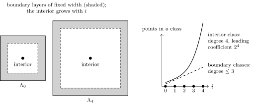
|
Figure 11. The five reflected tori \(\Lambda_i\) of Lemma 13.7, of sides \(2 (w + i)\), drawn for \(i = 0\) and \(i = 4\). A point \(y\) of \(\Lambda_i\) is classified by its distance, through the read radius \(R\), from each reflection face; at the shifted configurations \(V_{i, x - \tilde{y}}\), healthy near \(x\), the local formula takes the same value on a class for all \(i\). The boundary layers have fixed width, so a boundary class has a number of points of degree at most three in \(i\), while the interior class grows, with degree four and leading coefficient \(2^4\). The fourth difference \(\sum_i (- 1)^i \binom{4}{i} (\cdot)\) annihilates degrees below four, so it removes every boundary class from the total and keeps the interior one. The tori are auxiliary evaluation domains, not physical volumes, and the cancellation takes place in the sum over all points, not term by term. |
Write \(f_a^0\) for a regular summand of the negative logarithm in
| \(\displaystyle \lambda_i = \frac{(- 1)^i \binom{4}{i}}{2^4 \hspace{0.17em} 4!}, \qquad G_x (V) = \sum_{i = 0}^4 \lambda_i \sum_{y \in \Lambda_i} F^{(i)}_y (V_{i, x}) \hspace{0.17em} .\) | (13.6) |
Here \(F^{(i)}\) is the same finite local formula on the auxiliary torus, with its value at \(1\) subtracted at each site. The mask discrepancy and the constant of the redistribution are
where \(\tilde{y}\) is the integer representative used in the reflection.
For the estimates below put \(\mathfrak{b}= \hat{\beta}_{m + 1}\); \(P_j\) has subpower growth.
Lemma
Each \(L_x\) reads only links and flags in \(N_{2 \bar{w}} (x)\) and vanishes when that set is healthy, and
Proof. The identity is a rearrangement; the
vanishing of \(L_x\) is the fourth-difference cancellation; the bound on
\(G_x\) comes from the auxiliary logarithm, estimated with the classical
and one-loop subtractions of Section 12. Summing
Use the polynomial period requirement in item 7 of Table 3, in addition to \(100 (B + 1) \leqslant L_p D_m\). Write \(n = L_p D_m\). The radius \(R\) of the local construction is affine in \(B\) with stage-dependent coefficients, computed from the low-order radius; hence \(\bar{w} = 4 R + 100 (1 + B) + 5\) is affine in \(B\) with positive coefficients. Put \(\bar{a} = 2 \bar{w} |_{B = 1}\). The chosen stage has integers \(v_j^{\text{per}}, h_j^{\text{per}}\) with \(v_j^{\text{per}} \geqslant \bar{a}\), \(h_j^{\text{per}} \geqslant 1\) and
These are the minimum-period choices made after the ratios. Since \(B \geqslant 1\),
The reflection cubes, whose side is at most \(2 (w + 4) < 2 \bar{w}\), therefore embed, as does every radius-\(R\) read set. The larger health set \(N_{2 \bar{w}} (x)\) is a set on the original torus and need not embed; the argument uses only its containment of the queried links and flags.
For the local comparison, suppose that the field is healthy on the radius-\(R\) neighbourhood. Translate its cube to \([0, 2 R]^4\). On integer representatives \(0 \leqslant k < n\), fold each coordinate by \(q (k) = k\) for \(k \leqslant 2 R\), \(q (k) = 4 R - k\) for \(2 R < k \leqslant 4 R\), and \(q (k) = 0\) thereafter. Pull back links along this map, reversing them on decreasing edges and setting them to the identity on collapsed edges. A plaquette becomes a plaquette of the original cube, with possible reversal and conjugation, or has identity holonomy. The field is therefore globally healthy and agrees with the original field on the cube. The bound \(4 R < n\) permits the construction without a divisibility assumption on \(n\). Locality then permits this replacement when comparing the common local formulas on different periods.
We verify the vanishing of \(L_x\) on a healthy \(N_{2 \bar{w}} (x)\).
The complete read supports then lie in that set, every mask in
Classification of the terms. Here are the quantitative estimates on the sum before this localization. Put \(\mathfrak{b}= \hat{\beta}_{m + 1}\) and \(\mathfrak{h}=\mathfrak{b}^{3 / 8}\). In the convergent connected sums multiply the majorant of each ordinary elementary factor by \(\mathfrak{h}\). The rooted attachment parameter still tends to zero, since \(\mathfrak{h}\mathfrak{b}^{- 7 / 16} =\mathfrak{b}^{- 1 / 16}\). A term with at least three such factors across its polymers gains \(\mathfrak{h}^{- 3}\) upon restoring its original weights. A term with a retained large-field overlap has the same gain because its suppression is at least \(\mathfrak{h}^{- 3}\). The sum after multiplication has size at most a subpower factor times \(\mathfrak{h}\mathfrak{b}^{- 7 / 16}\). Thus the terms in these two classes have bound
| \(\displaystyle P_j (\mathfrak{b}) \mathfrak{h}^{- 3} (\mathfrak{h}\mathfrak{b}^{- 7 / 16}) = P_j (\mathfrak{b}) \mathfrak{b}^{- 19 / 16} \leqslant \mathfrak{b}^{- 23 / 20}\) | (13.8) |
after the coupling threshold is raised. The reserve is \(19 / 16 - 23 / 20 = 3 / 80\). This estimate also bounds fixed ordered derivatives: their placement polynomial was included before the rooted sum.
The connected sum separates into three parts. First retain the inherited
terms using Lemma 13.6; their principal sum is made smaller
than a prescribed multiple of \(\epsilon^{\text{pre}}_m\) by choosing
the ratio, and their comparison remainder by raising the threshold.
Among all other connected terms retain also those whose total support
size exceeds the low-order radius: their support decay is at most
\(\mathfrak{h}^{- 3}\) after the threshold is raised, so the estimate in
The auxiliary logarithm. For the finite sum use the stationary integral on each \(\Lambda_i\). Their sides \(2 (w + i)\) satisfy \(2 (w + i) \geqslant 100 (B + 1)\). The entry choice \(B \geqslant j + 4\) also gives \(\ell_m \hspace{0.17em} 2 (w + i) \geqslant 100 ((j + 3) \ell_m + 1)\) for their fine periods. Thus the coarse-period form of Lemmas 11.12–11.14 applies, without requiring these auxiliary periods to belong to the chosen physical-volume sequence. Subtract its flat value and the classical cubic, quartic and quadratic one-loop terms of Lemmas 12.6–12.9. Differentiation of its logarithm gives connected expectations under the common Gaussian law. For the terms not involving incoming errors, write the normalized local integral as \(\mathbb{E} \exp (V_3 + V_4 + V_{\geqslant 5})\), after the stationary action and its Gaussian determinant have been extracted. The subscripts refer to the Taylor degree in the link chart. Gaussian parity removes a lone odd cubic term. The fourth-order stationary terms are already in the classical path action, and the field-dependent quadratic part of the determinant is already in \(\alpha \mathcal{Q}_m\) and the quadratic loop atoms. Subtracting the value at \(1\) removes the remaining vacuum terms. Expanding \(\log \mathbb{E}e^V\) through two factors gives \(\mathbb{E}V + \frac{1}{2} (\mathbb{E}V^2 - (\mathbb{E}V)^2)\); its remaining terms have at least three factors. In normalized fluctuation coordinates each nonquadratic factor starts at order \(\mathfrak{b}^{- 1 / 2}\). The common Gaussian majorant bounds the last terms by \(P_j (\mathfrak{b}) \mathfrak{b}^{- 3 / 2}\). In the one- and two-factor terms that remain after the stated cancellations, Taylor's integral remainder and the healthy field bound give
Every radius and chart loss is included in the subpower factor. Each of
the four power terms has exponent at most \(- 3 / 2\) before that
factor; the path exponential decreases faster than any fixed power.
Terms involving incoming activities are not low-order; apart from the
inherited terms they obey
| \(\displaystyle C_j \mathfrak{b}^{- 23 / 20} + 2 | \Lambda_i | \{C_j \mathfrak{b}^{- 23 / 20} + \varepsilon_{\text{tr}} \} \hspace{0.17em} .\) | (13.9) |
Here \(\varepsilon_{\text{tr}} > 0\) is the chosen truncation error. The first term is the centered local integral; the two volume terms bound the omitted regular sum at the field and at \(1\). Approaching a boundary point of the healthy domain by radial contraction preserves these estimates, so they hold on the closed domain used in Definition 5.3.
A direction of that definition, restricted to \(N_{\bar{w}} (x)\) and
reflected, is bounded by \(2 t (1 + \bar{w})^{\varpi_{J_m}}\). Rescaling
each of at most \(\mathfrak{q}_{J_m}\) directions in
All the factors outside the negative powers are fixed powers of \(1 +
B\). Also \(\text{cov}_B (N_{\bar{w}} (x))\) is bounded by a stage
constant. The regular bound divided by \(\epsilon_m^{\text{reg}}\) tends
to zero, since \(23 / 20 > 11 / 10\). Finally,
To specify the small coefficient, let \(C_j^{\text{sub}}\), \(C_j^{\text{low}}\) and \(C_j^{\text{high}}\) be the operator bounds for local subtraction, low path replacement and the part of high path replacement proportional to \(\epsilon^{\text{pre}}_m\). These are the three linear operations in the following subsections; they are fixed from the output derivative norm and path bounds. Put \(C_j^0 = C_j^{\text{sub}} + C_j^{\text{low}} + C_j^{\text{high}}\). These constants use only derivative orders, direction powers, support exponents, and the output path bounds. For a prescribed \(0 < \theta \leqslant 1\), choose before the ratios
The quantity \(\epsilon^{\text{pre}}_m\) depends on \(m\) through
\(\epsilon_m^{\text{reg}}\). The next assertion concerns the very same
block integral and the masks of
Lemma
with \(\kappa_j^{\text{pre}} > 0\) fixed after the ratio. Restricting the interval preserves all this.
Proof. The connected expansion of Lemma 13.5
supplies the terms, Lemma 13.6 and the classification in
the proof of Lemma 13.7 bound all but the low-order ones,
and Lemma 13.7 localizes the latter; the choices below
split \(\epsilon^{\text{pre}}_m\) among them. First choose the ratio so
that the inherited principal terms of Lemma 13.6 use at
most \(\epsilon^{\text{pre}}_m / 32\), and then raise the threshold so
that their comparison remainders use at most \(\epsilon^{\text{pre}}_m /
32\). Bound the terms retained in
Next fix the truncation index. The low-order tail reads only the
prescribed path, the coupling and the incoming addresses. For each
coupling in \(\mathfrak{B}_{m + 1}\) summability gives a tail smaller
than \(\varepsilon_{\text{tr}} / 2\); weighted continuity in the
coupling gives a neighbourhood on which the same tail is smaller than
\(\varepsilon_{\text{tr}}\). Finitely many neighbourhoods cover the
compact \(\mathfrak{B}_{m + 1}\); take the largest index. This index
depends only on the incoming address lists, so it serves every input
with these lists. Increasing the index preserves the tail bound. Choose
the tail bound to be at most \(\epsilon^{\text{pre}}_m / 16\). The
regular terms outside the finite sum then have total at most \((1 / 16 +
2 / 16) \epsilon^{\text{pre}}_m\). Choose \(\varepsilon_{\text{tr}}\) so
that the two localization errors in
The change in the scalar is \(\tau_u^{\text{old}} - F_0 (1)\), with the
sign fixed by
for some \(\kappa_j^{\text{pre}} > 0\), since \(\beta'_u \geqslant \hat{\beta}_{m + 1} / 2\). One extra support power is used in this collection, leaving \(\sigma + 1\). Lemma 13.4 proves the asserted site bound and absolute convergence. No scalar depends on the output configuration, and all identities hold also when a chord is exactly at a threshold.
For continuity, the truncation and all reflected tori are now fixed. Finite linear combinations preserve the weighted comparison from Lemma 13.5. A difference of forced products has one marked difference factor; the rooted sum has the same strict attachment margin. Dominated convergence proves the weighted comparison after the collection. Flat evaluation gives continuity of the scalar. The support enlargement, inventories and conjunctions of tests are fixed. The same constructions commute with translations and signed permutations by reindexing. Every assertion is pointwise in the interval parameter or a convergence assertion within the interval, so restriction to a closed subinterval preserves it.\(\Box\)
The preparatory regular sum is \(E_u^{\text{pre}} = \sum_i f_{i, u}\) on the healthy domain. Its weighted bound is the anchored sum of Definition 5.4, before flat-value and Hessian subtraction. The next identity supplies the scalar reset.
Lemma
In particular \(\mathcal{H}_u (1), \mathcal{H}_u (U) > 0\) on this set.
Proof. Restrict the identity
The subtraction is local and uses no bound on the eventual coupling
correction. It extracts from each preliminary regular function its
response to constant curls, written with the clover curvature of
For a preliminary \(f\) on \(X\) anchored at \(o\), put \(Z = X \cup N_2 (o)\). For \(q = (a, b)\) and \(T \in \mathfrak{g}\), set \(A^{q, T}_{(y, c)} =\boldsymbol{1}_{c = b} \xi_o (y)^a T\), and fix a unit vector \(T_{\ast} \in \mathfrak{g}\). Define
Set \(q_f = 0\) when \(Z\) wraps. The matrix extracts the response to constant curls; its color independence is proved below. Define the regular remainder and the discrepancy of masks by
The following identity is checked before any activities are summed.
Lemma
The function \(R_f\) is regular on \(Z\), vanishes at \(1\), and has zero affine Hessian when \(Z\) is nonwrapping. The Borel gauge-invariant function \(\zeta_f\) depends only on internal links and flags in \(Z\) and vanishes when \(Z\) is healthy.
Proof. Gauge invariance reduces the affine
Hessian to its response to constant curls, Schur's lemma makes that
response colour-independent, and the clover formula
For each pair of orientations the colour form \((S, T) \mapsto D^2 [f (\exp \cdot)] (0) [A^{q, S}, A^{r, T}]\) is \(\text{Ad} (G)\)-invariant. The complexified adjoint representation of the compact simple Lie algebra \(\mathfrak{g}\) is irreducible, so every invariant bilinear form on \(\mathfrak{g}\) is a multiple of the trace form (Schur's lemma); testing on \(T_{\ast}\) identifies the multiple.
The side satisfies \(L_p D_m \geqslant 100 (B_m + 1) > 20\), which
permits the clover loops and affine tests without degeneracies. Equation
All indicators in \(\zeta_f\) read flags in \(Z\). If \(Z\) is healthy, every mask in the identity is one and \(\zeta_f = 0\); the identity reduces to the definition of \(R_f\). If \(Z\) is unhealthy, \(h_Z R_f = 0\) and the definition of \(\zeta_f\) gives the identity directly. This proves the equality on every configuration and the stated locality and cancellations.\(\Box\)
The same subtraction has a quantitative bound. If \(a_f\) majorizes \(f\), the diagonal tests \(tA^{q, T_{\ast}}\) and their half-sum are permitted directions in Definition 5.3. They give
| \(\displaystyle t^2 |q_f (q, q) | \leqslant a_f, \qquad t^2 |q_f (q, r) | \leqslant 3 a_f \hspace{0.17em} .\) | (13.14) |
Indeed four times the half-sum's diagonal Hessian is \(t^2 (q_f (q, q) + q_f (r, r) + 2 q_f (q, r))\). Its absolute value and the two diagonal bounds give the second estimate. Product differentiation of the four-link formula bounds every permitted derivative of \(F^{\text{cl}}_q\) by \(C_j t\) at a healthy anchor. For order zero this follows from the plaquette chord bound; at positive order the direction factors supply \(t\), and all undifferentiated group matrices are bounded. Hence
| \(\displaystyle \|R_f \|_{m, Z} + \sup_U | \zeta_f (U) | \leqslant C_j a_f \hspace{0.17em} .\) | (13.15) |
For \(\zeta_f\), the terms \(Q_f\) and \(f\) occur only under their own relaxed threshold tests, so the estimates still apply when \(Z\) is unhealthy.
Enlargement costs at most \(\text{cov}_B (Z) \leqslant \text{cov}_B (X) + 1\): one radius-\(B\) ball centered at \(o \in X\) contains \(N_2 (o)\) and meets the original connected cover. Also \(\text{dist} (x, o) \leqslant CB \text{cov}_B (Z)\) for \(x \in Z\), by following the connected cover. For a support of covering number \(n\) through \(x\), its anchor lies within distance \(CBn\) of \(x\), giving at most \(C (1 + B)^4 (1 + n)^4\) possible anchors. The inequality \((1 + n)^4 \leqslant Ce^n\) converts exponent \(\sigma + 3\) at the anchor to exponent \(\sigma + 1\) at a site: one support power bounds this polynomial and one remains unused. At exponent \(\sigma\) the enlargement itself costs only a stage constant. Without these extra powers the conversion would leave a polynomial in \(n\) at the original exponent.
Sum \(q_{f_{i, u}}\) at each anchor. Translation covariance makes the result independent of the anchor. Reflection in an axis belonging to exactly one of two distinct orientations changes the sign of the off-diagonal entry, so that entry is zero. Permuting axes identifies the diagonal entries. Thus a single real \(\Delta_u\) satisfies
The coefficient sums converge absolutely by
Put \(\alpha = \alpha_{N, m}\). After Section 13.2 the exponent contains \(\alpha \mathcal{Q}_m + \frac{\Delta_u}{2} \sum_o h_{\{o\}} \sum_q |F^{\text{cl}}_q (U, o) |^2\), whereas the output density must contain \((\alpha + \Delta_u) \textsf{K}^{\text{kin}}_m\). The difference consists of clover versus plaquette curvature, the missing cubic and quartic atoms, and the clips and health masks. The first two become regular activities, \(e_{\lambda, u}\) below and \(- (\alpha + \Delta_u) \mathfrak{a}^{(k)}_i\); the third, \(\ell_{\lambda, u}\), vanishes on healthy supports and, with the mask discrepancies \(\zeta_f\) of Lemma 13.10, is absorbed into the forced activities by Lemma 13.11. Define
The regular function is used with mask \(h_{Z_{\lambda}}\). Its affine Hessian vanishes because its two terms have the same constant-curl response. Add also the regular cubic and quartic functions \(- (\alpha + \Delta_u) \mathfrak{a}_i^{(k)}\), with their prescribed masks; they have zero Hessian because \(k \geqslant 3\). Every \(\ell_{\lambda, u}\) vanishes on healthy \(Z_{\lambda}\).
Write the logarithmic corrections \(\zeta_{f_{i, u}}\) and \(\ell_{\lambda, u}\) as \(\ell_a\) on nonempty supports \(Z_a\). A connected selection \(P\) consists of preliminary forced labels and logarithmic labels, contains at least one forced label, and has pairwise disjoint preliminary forced supports. Connected means connected in the graph joining intersecting supports. Its support \(Y_P\) is the union of all supports, including logarithmic supports; its inventory \(I_P\) is the union of the preliminary forced inventories. Define
| \(\displaystyle K_P (U) =\boldsymbol{1}_{\{Y_P \cap \text{Flag}_m (U) = I_P \}} \prod_{i \in P_{\text{for}}} k_{i, u} (U) \prod_{a \in P_{\text{log}}} (e^{\ell_a (U)} - 1) \hspace{0.17em} .\) | (13.18) |
The extra test is the conjunction of the preliminary forced tests. Selections and tests are fixed as \(u\) varies.
Lemma
Then the exact-cover gas of
Proof. The identity is a regrouping of finite
selections into overlap components; the bound is Lemma 13.4.
Expand \(\exp (\sum_a \ell_a) = \prod_a (1 + (e^{\ell_a} - 1))\).
Decompose a finite selection, together with a selection from
\(\mathcal{F}_u^0\), into support-overlap components. A nonzero
logarithmic factor meets a flag. Exact coverage assigns that flag to a
preliminary forced label, whose support meets the logarithmic support.
Every component therefore contains a forced label. Their union supports
are disjoint; their union inventories cover all flags. Conversely the
components recover the original selection uniquely. The eligibility
indicator in
For the absolute bound retain \(e^{- \kappa_{\text{fus}}}\) from one forced label per connected selection. Apply Lemma 13.4, with \(\eta = 1\), to the weights \(\mathfrak{v}_i = v_i e^{\sigma \text{cov}_B (Z_i)}\); its hypothesis follows from \((2 B + 1)^4 \gamma \leqslant 1\) and the extra exponent in the hypothesis here. It bounds the rooted tree sums by \(\mathfrak{v}_i e^{\text{cov}_B (Z_i)}\), and the sum of these bounds over roots whose supports contain a fixed site is at most \(\gamma\). Every connected selection has a spanning tree rooted at a label whose support contains that site, so its sum is at most \(\gamma \leqslant e^{\gamma} - 1\). The covering number is subadditive on intersecting unions, which retains \(e^{\sigma \text{cov}_B (Y_P)}\) in this comparison. Restoring \(e^{- \kappa_{\text{fus}}}\) gives the claimed bound. The resulting summable envelope justifies passage from finite expansions to the infinite identity.\(\Box\)
Let \(E_u^{\text{sum}}\) be the masked sum of the \(R_{f_{i, u}}\), the \(e_{\lambda, u}\), and the cubic and quartic corrections. Let \(\mathcal{F}_u\) be the fused gas. Hold these functions fixed while a trial parameter \(\vartheta\) varies, and put
The parameter \(\vartheta\) is the free coupling correction of the scalar reset. Lemma 13.13 shows that \(\vartheta = \Delta_u\) gives the density identity at every configuration; at one healthy test configuration \(V\) with \(\textsf{K}^{\text{kin}}_m (V) > 0\), Lemma 13.14 uses the affine dependence on \(\vartheta\) to read off \(\Delta_u\), which gives its continuity in \(u\) and, with Lemma 12.9, the drift bound. The output representation is the following single list: regular addresses \((Z_i, o_i)\) with functions \(R_{f_{i, u}}\), addresses \((Z_{\lambda}, o_{\lambda})\) with functions \(e_{\lambda, u}\), the cubic and quartic addresses of Definition 12.1 with functions \(- (\alpha + \Delta_u) \mathfrak{a}_i^{(k)}\), and forced addresses \((Y_P, I_P, \mathcal{E}_P^{\text{extra}})\) with functions \(K_P\). Each regular function carries its own health mask. We prove the inequalities
| \(\displaystyle e^{- \kappa_{\text{fus}}} (e^{\gamma} - 1) \leqslant \epsilon_m^{\text{for}}, \qquad \mathcal{E}_m \leqslant \epsilon_m^{\text{reg}} \hspace{0.17em} .\) | (13.19) |
in Lemma 13.12 before using them for the density identity. They impose no condition on the trial coupling.
Lemma
Lemma 13.16 states the same bounds for the Wilson representation, and Lemma 13.17 extends them to all the chosen classes.
Proof for a coarse output. The regular bound
adds the costs of the three linear operations to the preparatory bound
of Lemma 13.8; the forced bound applies Lemma 13.11.
Equation
The constant \(c_j = [64 (1 + C_j^0)]^{- 1}\) was chosen before the ratios in Lemma 13.8. After the ratio is fixed, Lemma 12.9 bounds \(| \alpha |\); raise the entry threshold until \(C_j^1 | \alpha | t^3 \leqslant \epsilon_m^{\text{reg}} / 2048\). This is possible because \(t^3 / \epsilon_m^{\text{reg}} = \hat{\beta}_m^{- 2 / 5} (M^{\text{cut}}_m)^3 \to 0\). Take \(\theta \leqslant 1 / 32\) before the ratio. Since \(C_j^0 c_j \leqslant 1 / 64\), the sum is at most \(\epsilon_m^{\text{reg}} / 1024\). The same argument allows any prescribed smaller coefficient by choosing \(\theta\) first and raising the threshold for the second term.
For the logarithmic corrections, conversion from anchored sums to site
sums costs at most \(C_j (1 + B)^4\), after the extra support powers
pay the powers of the covering number. The local subtraction costs \(C_j
\epsilon^{\text{pre}}_m\). The low terms in
The linear clipped tail is bounded by \(2 c_{\text{lin}} t\) times its coefficient, since chords are at most two. For a failed relaxed threshold test, the remote threshold supplies \(e^{l / R_{J_m}^{\text{rel}}}\) in a path of length \(l\). It is paid by the path decay because \(R_{J_m}^{\text{rel}} w_{J_m}^{\text{path}} \geqslant 12\). The common-anchor clover term costs \(| \Delta_u | t^2 \leqslant \epsilon^{\text{pre}}_m\). These estimates give exactly the displayed bound, including unhealthy configurations. Since \(\epsilon^{\text{pre}}_m / t = O_j (\hat{\beta}_m^{- 3 / 5} / M^{\text{cut}}_m)\) and \(| \alpha |\) is fixed after the ratio, \((1 + B)^4 m_j \to 0\).
Let \(\kappa_{\text{fus}} = \kappa_j^{\text{pre}} (M^{\text{cut}}_{m +
1})^2 / 2\). The majorants in
Every address is a finite combination of countable preliminary and path
addresses, so the families are countable. Subtraction and path
replacement transport the entire address under translations. Signed
permutations transform the curvature orientations with their signs; the
finite group average includes every transformed term. These permutations
act on supports, anchors and functions. On a connected selection they
also transform the union inventory and conjunction of tests. Equation
The identity below fixes the whole density before the scalar estimate of Lemma 13.14. Its proof uses the bounds just established.
Lemma
Moreover \(\mathcal{F}_u (U) = 1\) when \(\text{Flag}_m (U) = \varnothing\).
Proof. Local subtraction rewrites the
preliminary regular functions, path replacement turns the masked
quadratic functional into the kinetic action, and fusion absorbs the
logarithmic corrections; the bounds
All sums converge absolutely. For each low term
Sum and apply
Lemma 13.11 incorporates the last two sums into \(\mathcal{F}_u\). Hence, on every configuration,
| \(\displaystyle \mathcal{H}_u (U) = e^{(\tau_u - c_u / | \Lambda |) | \Lambda |} q_{u, \Delta_u} (U) \hspace{0.17em} .\) | (13.20) |
At \(1\) all path and final regular terms vanish. The only exact-cover
forced selection is empty, so \(q_{u, \vartheta} (1) = 1\) for every
\(\vartheta\). Equation
The regular cancellations were proved in Lemma 13.10 and
after
The density identity of Lemma 13.13 holds with a value \(\Delta_u\) that the construction fixes before the bound on it proved here is used. The proof order is

Before the estimate below the following are available: the path arrays and \(\alpha_{N, m}\) (Section 12), the activity families with their bounds (Lemma 13.12), and the exact identity \(q_{u, \Delta_u} =\mathcal{H}_u /\mathcal{H}_u (1)\) (Lemma 13.13). Section 13.2 already gives \(t_m^2 | \Delta_u | \leqslant \epsilon^{\text{pre}}_m\), which the activity bounds use and which alone implies \(| \Delta_u | < 1\) and the drift bound. The estimate below is an alternative proof of \(| \Delta_u | \leqslant 1\) that uses the activity bounds but not the formula for \(\Delta_u\). The reset gives a second description of the same coefficient: evaluating the identity at one configuration with positive kinetic energy identifies \(\Delta_u\) as the unique root of an affine scalar equation. This explicit formula, with the continuity of Lemma 13.15 in Section 13.4 (whose proof does not use Lemma 13.14), gives the continuity of \(\Delta_u\) in \(u\); with Lemma 12.9 it gives the drift bound.
For an input curve \(\rho'_u\) of Theorem 5.5, recall \(\mathcal{H}_u =\mathcal{B}^{(m)}_{\beta'_u} \text{dens} \hspace{0.17em} \rho'_u\), and put \(b_u = \beta'_u + \alpha_{N, m}\). Lemma 13.13 supplies regular and forced sums \(E_u^{\text{sum}}, \mathcal{F}_u\), independent of \(\vartheta\), with trial density
the flat-field normalizations \(q_{u, \vartheta} (1) = 1\), and \(q_{u,
\Delta_u} =\mathcal{H}_u /\mathcal{H}_u (1)\). Lemma 13.9
gives a preparatory sum \(E_u^{\text{pre}}\) with bound \(c_{\text{pre}}
\epsilon_m^{\text{reg}} / 4\), for a stage constant \(c_{\text{pre}}
\geqslant 4\), and Lemma 13.12 gives the final bound
Lemma
The bound is independent of \(N, p, u\) and the input curve.
Proof. We evaluate the exact identity of Lemma 13.13 at one configuration \(V\) with kinetic energy of order \(| \Lambda | t_m^2\); the identity is affine in the reset, which is then read off. Recall \(t = t_m \leqslant 1\) from item 7 of Table 3. Put a group element of chord \(h_V = \tau t\) on direction-\(1\) links whose second coordinate is even, and the identity elsewhere. Continuity along a nonconstant one-parameter subgroup gives \(\varepsilon_G > 0\) such that every chord in \([0, \varepsilon_G]\) occurs. Choose
Every \((1, 2)\) plaquette has chord \(h_V\) and all other plaquettes have chord zero. Thus this configuration \(V\) is everywhere healthy. All periods here are even because \(4 \mid L_p\). Signed permutations permute the plaquettes and preserve their chords, so the direct contribution to \(\textsf{K}^{\text{kin}}_m (V)\) is at least \(| \Lambda | c_{\text{dir}, J_m} h_V^2 / 2\). Row squares are nonnegative. Since \(| \text{proj}_{\mathfrak{g}} (U - U^{- 1}) / 2| \leqslant \text{ch} (U)\) and adjoint transport is isometric, every slot has norm at most \(h_V \leqslant 1 / 4\). Lemma 12.3 bounds the absolute sum of cubic and quartic terms by
Each signed image of \(V\) has the same plaquette chords with a single nonzero orientation. Hence the bounds apply to every term of the hypercubic average. Consequently
Lemma 13.9 gives \(\mathcal{H}_u (1), \mathcal{H}_u (V) > 0\). Put \(v_u = | \Lambda |^{- 1} \log \mathcal{H}_u (1)\). Taking the logarithmic contrast in Lemma 13.9 gives
The pre-reset bound of Lemma 13.9, summed over anchors as in Definition 5.4, bounds each of the last two values by \(| \Lambda | c_{\text{pre}} \epsilon_m^{\text{reg}} / 4\). No vanishing condition at \(1\) is needed for this preparatory sum.
On everywhere-healthy configurations every curvature slot has norm at most \(t\). Lemma 12.3 and \(t \leqslant 1\) therefore give
After \(\ell\) is fixed, Lemma 12.9 bounds \(| \alpha_{N,
m} |\) by a stage constant. Raise the coupling entry threshold until \(2
| \alpha_{N, m} | A_{J_m}^{\text{path}} t^3 \leqslant
c_{\text{pre}}
\epsilon_m^{\text{reg}} / 2\). This is possible since
\(t^3 / \epsilon_m^{\text{reg}} = \hat{\beta}_m^{- 2 / 5}
(M^{\text{cut}}_m)^3
\to 0\). Together with
For the final regular sum, Lemma 13.12 and
Since the activity families are fixed as \(\vartheta\) varies, the scalar discrepancy is affine:
Since \(V\) has no flagged sites, \(\mathcal{F}_u (V) = 1\). Evaluating the exact identity of Lemma 13.13 at \(V\) gives \(f (u, \Delta_u) = 0\). As \(K_V > 0\), this determines
Increase the entry threshold to obtain the final inequality, using \(\epsilon_m^{\text{reg}} / t_m^2 = \hat{\beta}_m^{- 1 / 10} (M^{\text{cut}}_m)^{- 2} \to 0\). The block integral and activity sums are continuous in \(u\) by Lemma 13.15 of Section 13.4, whose proof does not use the present lemma; so \(\Delta_u\) is continuous.
Multiplication by \(\mathcal{H}_u (1) = e^{v_u | \Lambda |}\) gives the density identity at \(\Delta_u\). Its coupling is \(\beta_u = \beta'_u + \alpha_{N, m} + \Delta_u\). Lemma 12.9 and \(| \Delta_u | \leqslant 1\) prove the claimed drift.\(\Box\)
The scalar reset of Lemma 13.14 and the step on curves need continuity of the integral and both final sums. The next deduction uses the weighted comparison in Lemma 13.8 and does not use Lemma 13.14.
Lemma
are continuous.
Proof. Every operation of the step is linear at
fixed addresses or a convergent product with a strict attachment margin,
so the weighted continuity of Lemma 13.8 carries over. The
maps \(f \mapsto f (1), q_f, R_f, \zeta_f\) are linear on functions with
fixed address. Equation
For fusion each coefficient is a finite product and hence continuous in supremum norm. To justify summing weighted differences, work first along subsequences with one summable majorant. Given \(u_n \to u_0\), pass to a subsequence whose total weighted preliminary discrepancies are at most \(2^{- n} \varepsilon\). Add their nonnegative majorants to those at \(u_0\); the extra mass is at most \(\varepsilon\). The margin \((2 B + 1)^4 \gamma \leqslant 1 / 2\) arranged in the proof of Lemma 13.12 permits this addition for small \(\varepsilon\). Lemma 13.11 gives one summable envelope for the fused coefficients along this subsequence. Dominated convergence gives convergence of their weighted differences. If the original sequence failed to converge, a subsequence with discrepancies bounded away from zero would admit such a further subsequence, a contradiction. This proves weighted continuity without assuming a common envelope on an arbitrary neighborhood. Constants here may depend on the fixed volume.
For the pointwise gas, put \(M_i = \max (\sup |K_{i, u} |, \sup |K_{i, u_0} |)\). Telescoping finite products and summing selections gives
The restrictions on exact coverage use fixed inventories. Weighted continuity makes the right side tend to zero. The regular sum is continuous by the analogous sum of order-zero differences. The same bounds give continuity in \(u\), uniform in \(U\), for the input density at fixed volume, since its path action is affine in the continuous coupling.
Finally the kernel of Definition 5.1 is uniformly bounded on a compact coupling interval at this volume. The tag masses sum to one; its single-link normalizing integrals are positive and continuous in the coupling, and its link factors are bounded on the compact group. Dominated convergence against product probability Haar measure gives continuity of \(\mathcal{H}_u (U)\). This proves all three pointwise continuities and weighted continuity, by Lemma 13.8.\(\Box\)
At the finest level the identity free form permits a local choice. Put \(\delta_{\text{dir}} = c_{\text{dir}, J_N}\) and \(F (u) = \text{proj}_{\mathfrak{g}} (u - u^{- 1}) / 2\). To define the quartic term, let \(\psi\) be the local inverse of \(X \mapsto F (e^X)\) at zero and set
The inverse exists since \(DF (e^{\cdot}) (0) = I\). This invariant quartic polynomial is chosen so that
| \(\displaystyle R (u) = \text{pr} (u) - \tfrac{1}{2} |F (u) |^2 - T_4 (F (u))\) | (13.22) |
has zero Taylor terms through degree four at \(1\). This is the case \(m = N\) in the proof of Lemma 12.6. The path action of Definition 12.2 at \(m = N\) has row \(\sqrt{1 - \delta_{\text{dir}}} \hspace{0.17em} F\), no cubic or loop terms, and quartic term \((1 - \delta_{\text{dir}}) T_4 (F)\) with its prescribed mask. These finite path sums satisfy Lemma 12.3.
The initial activities retain the difference between Wilson energy and this action also on flagged configurations. The proof constructs the full curve.
Lemma
Its activity families are countable and equivariant, with majorants satisfying \(\mathcal{E}_N \leqslant \epsilon_N^{\text{reg}}\) and \(\mathcal{K}_N \leqslant \epsilon_N^{\text{for}}\), and the curve is continuous in the sense of Definition 13.3.
Proof of the initialization identity, bounds and continuity. The Wilson energy is split exactly into the path action of level \(N\), a fifth-order regular remainder, and a nonnegative unassigned action that is charged to the flags. Everything here is at level \(N\): \(j = J_N\), \(t = t_N\), \(B = B_N\) and \(\sigma = \sigma_{J_N}\). For a plaquette \(q\), write \(k_q^{\text{kin}} = (1 - \delta_{\text{dir}}) |F (U_q) |^2 / 2\), \(h_q = h_{\text{vertices} (q)}\), and \(\chi_q\) for its relaxed threshold test. Define its unassigned action by
The relaxed threshold test \(\chi_q = 1\) implies \(\text{ch} (U_q) \leqslant t\). The identity \((u - u^{- 1}) / 2 = (u - 1) (1 + u^{- 1}) / 2\) and contraction of the projection give \(|F (u) | \leqslant \text{ch} (u)\). Together with \(\text{ch} (u)^2 = 2 \text{pr} (u)\) this gives \(\mathcal{W}_q \geqslant 0\). For \(\text{ch} (U_q) > t\), \(c_{\text{lin}} < \delta_{\text{dir}} / 16 \leqslant 1 / 16\) gives \(\mathcal{W}_q \geqslant \text{ch} (U_q)^2 / 4 \geqslant t^2 / 4\). Substitution in the two cases gives
| \(\displaystyle \text{pr} (U_q) = L_q (U) + (1 - \delta_{\text{dir}}) h_q T_4 (F (U_q)) + (1 - \delta_{\text{dir}}) h_q R (U_q) +\mathcal{W}_q (U) \hspace{0.17em} .\) | (13.23) |
Here \(L_q\) is the direct clipped term plus the threshold-tested row square. The identity includes small plaquettes next to a flag and both sides of the clipping threshold.
Take the regular activities \(\beta (1 - \delta_{\text{dir}}) R (U_q)\) on their plaquette supports, anchored at the starting vertex, with the signed average of the path action. They vanish at \(1\) with their Hessians. Through the prescribed order their normalized healthy derivatives are bounded by \(C_j \beta t^5\). To verify this without assuming small links, use the plaquette holonomy as one coordinate and the other three links as compact parameters. The remainder vanishes to order five in the holonomy chart. At derivative order \(k \leqslant 5\), Taylor's formula leaves order \(5 - k\) and the direction factors supply \(t^k\). For \(k > 5\), bounded derivatives and \(t^k \leqslant t^5\) give the same estimate. The four-link formula controls the remaining compact factors. There are finitely many plaquettes at each anchor, so the regular sum is at most \(C_j \beta t^5\). On the top band,
Increasing the entry threshold gives the regular bound \(\epsilon_N^{\text{reg}} / 1024\) uniformly in volume.
Let \(\mathfrak{F}= \text{Flag}_N (U)\). Join two flags when their radius-\(2 B\) neighborhoods overlap. For each nonempty connected inventory \(I\) use \(Y_I = N_{2 B} (I)\) and
The charge \(d_I\) is the signed average of those \(\mathcal{W}_q\) whose anchors lie within distance \(B\) of \(I\), in the coordinates of that signed image. Every nonzero \(\mathcal{W}_q\) is assigned: a failure of the relaxed threshold test has a witnessing flag within this distance, since \(t \exp ((B - 2) / R_{J_N}^{\text{rel}}) \geqslant 2\). The other cases already meet a flag at a plaquette vertex. The anchors lie within \(B\) of \(I\), and each nonautomatic relaxed threshold test reads within \(B - 2\) of its anchor. Thus \(N_{2 B} (I)\) contains every link and flag used in the charge. Distinct actual components have disjoint supports, so each nonzero term is assigned once. Hence the sum of the component charges is the signed average of \(\sum_q \mathcal{W}_q\).
Every flag touches a plaquette with \(\text{ch} (U_q) > t\), and a plaquette has at most four vertices. Retaining the identity orientation in the nonnegative signed average gives
A nonzero exact-cover product of \(K_I\) selects precisely the overlap
components of \(\mathfrak{F}\). Indeed any two flags in one selected
connected inventory are connected in \(\mathfrak{F}\). Conversely a flag
joined to a selected inventory cannot lie in another selected inventory,
since their radius-\(2 B\) supports would intersect. Exact coverage then
forces every component to be selected. The actual components satisfy
eligibility. Thus the forced sum has exactly one nonzero term, equal to
the exponential of minus \(\beta\) times the unassigned action. Equation
For the forced norm, a connected inventory of \(r\) sites is encoded by a rooted spanning walk of length at most \(2 (r - 1)\) in the overlap graph. Each step has at most \(C (1 + B)^4\) choices, and \(\text{cov}_B (N_{2 B} (I)) \leqslant 5^4 r\). Counting possible roots for a support through a specified site costs another \(C (1 + B)^4\). With \(c = 1 / (16| H_4 |)\), the weighted sum is therefore bounded by
The top band gives \(\beta t^2 \geqslant (M^{\text{cut}}_N)^2 / 2\). This dominates both \(\log (1 + B)\) and the exponent in \(\epsilon_N^{\text{for}}\), so the geometric sum is eventually at most \(\epsilon_N^{\text{for}} / 1024\), uniformly in volume. Both normalized bounds can be made arbitrarily smaller by increasing the entry threshold.
Addresses and tests are independent of \(\beta\). Regular differences have the same majorants with \(\beta\) replaced by \(| \beta - \beta_0 |\). For the forced functions \(d_I \geqslant 0\) is bounded at fixed volume and
There are finitely many subsets of this torus, so the weighted difference sums tend to zero. Translations and signed permutations transport complete plaquette terms, component supports, inventories and tests. This gives covariance as well as continuity. We have proved the Wilson representation, both bounds, and its full continuous curve with scalar zero. The one-step assertion for the later levels is proved in Section 13.6.\(\Box\)
The shooting argument of Section 14 restricts parameter intervals repeatedly, so the step must be a fixed construction on curves that is compatible with restriction. We therefore fix, once for each continuous input curve, all choices of Sections 13.1–13.3: the tree gauge, the address identifications, the truncation index and the auxiliary tori; the last two depend only on the incoming address lists. The step on a closed subinterval is the restriction of the step on the larger interval. The estimates used to repeat the step are the following explicit ones. At level \(m\) the path is the fixed \(P^{\text{path}}_{N, m}\) of Definition 12.2, with the bounds of Lemmas 12.3–12.4. The activity functions satisfy Definitions 13.1–13.2 and Lemma 13.12. At an adjacent pair the output is exactly the functions in Lemma 13.13, its scalar is \(| \Lambda |^{- 1} \log \mathcal{H} (1)\), and its correction obeys
The first three bounds precede the scalar reset; the last is Lemma 13.14, and it also follows from the first. The input coupling belongs to \(\mathfrak{B}_{m + 1}\); no output-band condition is imposed.
The classes are defined inductively from the Wilson start. Put
\(\mathcal{I}_{N, p} = \{\rho^{\text{W}}_{\beta} : \beta \in
\mathfrak{B}_N \}\), with the curve of Lemma 13.16, and
\(\mathcal{A}_{N, N, p} =\mathcal{I}_{N, p}\). For \(m < N\), a
representation \(\rho\) at level \(m\) belongs to \(\mathcal{A}_{N, m,
p}\) if there are \(\rho' \in \mathcal{A}_{N, m + 1, p}\) with \(\beta'
= \beta (\rho') \in \mathfrak{B}_{m + 1}\) and a real \(\Delta\) with
\(t_m^2 | \Delta | \leqslant \epsilon^{\text{pre}}_m\) such that: the
path of \(\rho\) is \(P^{\text{path}}_{N, m}\); its regular activities
satisfy Definition 13.1 and are produced by local
subtraction and path replacement, and its forced activities satisfy
Definition 13.2 and are produced by fusion (Lemma 13.11),
from preliminary families with the properties of Lemma 13.8,
including
Lemma
Proof. The Wilson start (Lemma 13.16) supplies the initial curve and both caps; Sections 13.1–13.4 construct the step on a curve and prove its bounds, identity and continuity. At a step, Lemma 13.8 uses only the prescribed paths, the local regularity and forced eligibility, the bounds and the weighted continuity of its input, so the input curve need not coincide with an earlier chosen curve. Its truncation index depends only on the incoming address lists, so the same selection serves every input curve with these lists. Local subtraction, path replacement and fusion preserve the read supports, gauge invariance, cancellations and countability. Lemma 13.12 proves their numerical bounds, and Lemma 13.15 proves weighted continuity on the interval.
The normalized identity of Lemma 13.13 and the reset of
Lemma 13.14 identify the same \(\Delta\). Lemma 13.14
identifies \(\Delta\) with the continuous scalar root and gives \(|
\Delta | \leqslant 1\) and the drift in Theorem 5.5.
Defining the scalar normalization by flat evaluation gives the exact
integral, since the normalized representation is one at \(1\). Hence
every output is a member of the next class,
Restricting a chosen step to a closed parameter subinterval preserves its supports, tests, weighted continuity and estimates; weighted continuity becomes continuity in the relative topology of the smaller interval. We use this restricted step whenever the input curve is restricted. The construction applies to every continuous curve in the classes, regardless of how that curve was obtained. Thus the classes are closed under the step and under interval restriction, as required for the shooting argument in Section 14. Lemma 13.23 supplies the analytic estimates for this same recursion.\(\Box\)
Proof of Theorem 5.5. The step is the construction of Sections 13.1–13.3 applied to the input curve. Lemmas 13.9, 13.12, 13.13 and 13.15 give the final functions and their exact normalized identity. Put
The denominator is positive by Lemma 13.9. Lemma 13.15 gives continuity of \(v_u\) and of the activity families. Lemma 13.14 identifies this same \(\Delta_u\) with its continuous scalar root, and its drift estimate gives
Define \(\rho_u\) by these scalars and the activities in Definition 5.2. Multiply the identity of Lemma 13.13 by \(\mathcal{H}_u (1)\) to obtain \(\text{dens} \hspace{0.17em} \rho_u (U) =\mathcal{H}_u (U)\) for every configuration. Lemma 13.12 gives the activity caps and Lemma 13.15 gives continuity. Lemma 13.17 gives \(\rho_u \in \mathcal{A}_{N, m, p}\) and \((\rho_u, \rho'_u) \in \mathcal{R}_{N, m, p}\). The Wilson construction of Lemma 13.16 supplies the common initial curve with scalar zero.\(\Box\)
This subsection writes the specified recursion in coordinates \((\mathfrak{x}_m, A_m)\), a normalized coupling and the activities, and proves the following. The step maps are real-analytic on balls of fixed radius, with multilinear coefficients of degree at least one bounded by \(g_{\ast} = 1 / 128\) (Lemma 13.21). Hence the whole history is the unique fixed point of a contraction on power series in the endpoint coupling (Lemma 13.23), which gives endpoint tuning in Section 14. Each fixed-level coordinate converges along the full cutoff sequence (Lemmas 13.22 and 13.24), which drives the fixed-volume limit. Field differentiability does not give this parameter analyticity, because some activity functions are only measurable.
We compare cutoffs using activity functions on fixed domains. At level \(m\) and period \(p\), put all regular addresses into one countable list and all forced addresses into a second list. A missing term has coefficient zero. The lists contain every finite support, anchor and inventory used above, and every finite conjunction of their eligibility tests. The output of a fusion is indexed by its finite selection, so the lists are closed under the construction. Keep the same permutations for translations and signed permutations. This identifies different cutoffs without changing their health domains.
For a difference \(A = (E, K)\) of activity families set
The seminorms in this formula are the least majorants in Definitions 5.3–5.4. Quotient by zero seminorm and complete the space with the prescribed local cancellations, eligibility and permutations. Denote the resulting real Banach space by \(\mathcal{X}_{m, p}\). This retains regular derivatives on healthy configurations and forced values on every configuration. The scalar normalization is excluded.
The coupling coordinate must allow relative changes of \(\beta\) while keeping a uniform analytic radius. Define
Thus \(b_m\) converts a change of \(\mathfrak{x}_m\) into a change of \(\beta_m\), up to the factor \(2 \chi_m \mathfrak{x}_m\). Monotonicity gives \(b_m \geqslant \chi_0 \hat{\beta}_0 > 0\). Item 7 of Table 3 gives \(\bar{\beta} \geqslant 2^{224}\); then \(\chi_m \leqslant 1 / 128\). In the following paragraphs write \(b_{\min} = \chi_0 \hat{\beta}_0\), \(g_{\ast} = 1 / 128\) and \(\lambda_{\ast} = 1 / 16\).
Let \(F_{N, m}\) denote the selected activity map and \(\mathcal{D}_{N, m}\) its scalar correction, so that
The top map is denoted by \(F_N^{\text{W}} (\mathfrak{x}_N)\). The maps are constructed for \(\|A\| \leqslant 1\) and \(33 / 40 \leqslant \chi_m \mathfrak{x} \leqslant 47 / 40\). All inputs in this domain have the common address lists, so the truncation index and auxiliary tori of Lemma 13.8 are the same at every point. Hence \(F_{N, m}\) and \(\mathcal{D}_{N, m}\) are single-valued, and their restriction to a line is the construction on that line. We use expansions centred in the smaller domain
| \(\displaystyle \|A\| \leqslant 1 / 8, \qquad 17 / 20 \leqslant \chi_m \mathfrak{x} \leqslant 23 / 20 \hspace{0.17em} .\) | (13.27) |
A ball of radius \(1 / 4\) about such a centre stays in the larger
domain: its activity norm is at most \(3 / 8\), and the change of
\(\chi_m \mathfrak{x}\) is at most \(1 / 512 < 1 / 40\). For a retained
history with \(| \beta_0 - \bar{\beta} | \leqslant \bar{\beta} / 4\),
summing the drift and the error bound in Section 9 gives
\(| \beta_m - \hat{\beta}_m | \leqslant \hat{\beta}_m / 4\). Its square
root therefore lies in \([17 / 20, 23 / 20]\). Every activity in the
history, including the Wilson start, has norm at most \(1 / 1024\) by
the proofs of Lemmas 13.12 and 13.16. Thus the
entire history lies in
For a finite parameter evaluation formula with real weights \(c_{\nu}\) and nodes \(s_{\nu} \in [- 1, 1]\), define its moment bound
| \(\displaystyle \mathfrak{s} (c, s ; R) = \sup_{k \geqslant 0} \left| \sum_{\nu} c_{\nu} (s_{\nu} / R)^k \right| \hspace{0.17em}, \qquad R > 1 \hspace{0.17em} .\) | (13.28) |
It expresses analyticity through real evaluations: if \(f (s) = \sum_k a_k s^k\) with \(\sum_k \|a_k \| R^k \leqslant M\), then \(\| \sum_{\nu} c_{\nu} f (s_{\nu})\| \leqslant M \hspace{0.17em} \mathfrak{s} (c, s ; R)\), and Lemma 13.18 below proves a converse, up to halving the radius. The nodes lie on a parameter interval; they are unrelated to the spatial stencils of local fields.
Uniform line estimates at nearby centres control mixed finite differences; this supplies the multilinear coefficients for the endpoint equations.
Lemma
whenever \(\|h\| \leqslant r\) and \(4 e \|h\| < rR\). The \(T_k\) extend with the same bounds to the completion of \(X\).
Proof. Associate to a parameter evaluation formula the sequence \((\sum_{\nu} c_{\nu} (s_{\nu} / R)^k)_{k \geqslant 0}\) with supremum norm. The assumed inequality defines a bounded linear map, of norm at most \(C\), from their span to \(Y\). Extend it to the closure. The \(k\)th coordinate vector lies in that closure: the \(k\)th finite difference at \(0\), divided by \(k! (a / R)^k\), has zero moments below \(k\), moment one at \(k\), and higher moments tending uniformly to zero as its mesh \(a \to 0\). To see the uniformity, split the higher moments at any fixed order and use \(|ja / R|^n \leqslant (ka / R)^n\) for the remaining tail. Evaluation on a single point then gives the exact line series. Its coefficient sum at radius \(R / 2\) is at most \(2 C\). Uniqueness follows by successively dividing a vanishing series by its first possible power.
Write \(P_k (h)\) for the coefficient of \(s^k\) in \(f (x + sh)\). Rescaling \(s\) gives \(P_k (ah) = a^k P_k (h)\) and
We must prove the polynomial identity in the direction \(h\). Put \(\delta_h g (a) = g (a + h) - g (a)\). Uniform line remainders at nearby centres imply
Indeed insert the line series at \(x + sa\) into the \(n\)th forward difference. The coefficients below degree \(n\) cancel by \(\sum_{j = 0}^n (- 1)^{n - j} \binom{n}{j} j^k = 0\) for \(k < n\); the uniformly bounded tail is \(O (s^n)\).
For \(h_0, \ldots, h_{n - 1}\) and \(T \subset \{0, \ldots, n - 1\}\) set
There is the exact mixed-difference identity
| \(\displaystyle \delta_{sh_0} \cdots \delta_{sh_{n - 1}} f (x + sa) = \sum_T (- 1)^{n - |T|} \delta_{sv_T}^{\hspace{0.17em} n} f (x + s (a + w_T)) \hspace{0.17em} .\) | (13.29) |
Expand the right side as a sum over its \(n + 1\) forward-difference points. At the point indexed by \(j < n\), pairing sets \(T\) differing by the index \(i = j\) cancels the terms, since that index has coefficient \((j - i) / (n - i) = 0\). At \(j = n\) the coefficient of each \(h_i\) is one, leaving precisely the left side. Hence every mixed \(n\)th difference above is \(O (s^n)\).
Expand each of its finitely many values in its line series at \(x\) and compare powers of \(s\). It follows that
For \(n = k + 1\) this makes the \(k\)th difference of \(P_k\) independent of its base point. Define
The identity \(\delta_{u + v} = \delta_u + \delta_v + \delta_u \delta_v\) proves additivity in each slot, since the extra \((k + 1)\)st difference vanishes. The displayed bound on \(P_k\) makes these additive maps locally bounded, hence continuous and real linear in each slot. The operators commute, giving symmetry. Homogeneity gives \(\delta_h^k P_k (0) = k!P_k (h)\), so their diagonal is the original line coefficient.
There are \(2^k\) terms in this polarization sum, and the argument in each has norm at most \(k\) on unit directions. Thus \(k^k / k! \leqslant e^k\) gives the stated operator bound. The diagonal series equals \(f (x + h)\) by the line recovery; the norm bound proves its convergence on the stated domain. Continuous multilinear maps extend uniquely through the dense inclusion into the completion, with unchanged norm.\(\Box\)
We evaluate the maps along lines \((\mathfrak{x}(s), A (s)) = (\mathfrak{x}+ sv, A_0 + sA_1)\), with \(|v| \leqslant 1\) and \(\|A_0 + sA_1 \| \leqslant 1\) for \(|s| \leqslant 1\). Supports, flag and threshold tests and local function domains are fixed along the line. Write \(F (s) = F_{N, m} (\mathfrak{x}(s), A (s))\) and \(\mathcal{D} (s) =\mathcal{D}_{N, m} (\mathfrak{x}(s), A (s))\). Let \(\mathcal{N}_{\text{pre}}\) be the anchored regular norm at exponent \(\sigma + 3\), before division by \(\epsilon_m^{\text{reg}}\) and before subtraction. Let \(\mathcal{N}_{\text{for}}\) be the corresponding forced site norm at exponent \(\sigma + 1\).
The coupling varies through a square of an affine function. The next estimate controls that dependence at a radius growing with the reference coupling; a bound at one fixed field-derivative order would not suffice.
Lemma
For any prescribed \(\theta_{\text{W}} > 0\), the Wilson map satisfies the analogous normalized estimate with radius \(\mathfrak{R}\) and bound \(4 \theta_{\text{W}}\) after the entry threshold is raised.
The proof keeps physical fields fixed and then applies the connected and localization operations.
Proof. The parameter coefficients of the connected expansion of Lemma 13.5 are bounded by the same rooted estimate, with the Gaussian rescaling expanded in convergent Neumann series; the five tori of Lemma 13.7 then act on these coefficients. Put \(\upsilon =\mathfrak{b}^{- 1 / 128}\) and raise the threshold until
| \(\displaystyle 128\mathfrak{R} \chi_{m + 1} \leqslant \upsilon \leqslant 1 \hspace{0.17em} .\) | (13.30) |
This is possible since \(1 / 256 - 1 / 32 + 1 / 128 = - 5 / 256 < 0\). Set \(\zeta = \chi_{m + 1} \mathfrak{x}\) and \(L = \zeta - 6\mathfrak{R} \chi_{m + 1}\). For \(|s| \leqslant 6\mathfrak{R}\),
The displayed margins follow from
To estimate parameter coefficients, use physical link variables in each sector integral. All flag, allocation, tag and chart tests are then independent of \(s\): their thresholds are \(t_{m + 1}\) and the prescribed stage constants, not \(\beta (s)^{- 1 / 2}\). Old measurable forced functions occur as \(K_0 + sK_1\) at the same physical links. Gaussian rescaling is used to estimate the coefficients, after these functions have been held fixed. Thus parameter coefficients do not differentiate their field arguments or any test.
Here is the coefficient bound for this change of Gaussian scale. For a positive local precision matrix \(\textsf{A}\) and affine source \(\textsf{b}_0\), put \(m_0 = - \textsf{A}^{- 1} \textsf{b}_0\) and \(Q (a) = \langle a - m_0, \textsf{A} (a - m_0) \rangle / 2\). This is the centred quadratic energy in the sector Gaussian density. The parameter occurs through \(\beta (s) Q\), its normalizing determinant, and the local stationary corrections. For a precision perturbation \(H\),
Both series are estimated through the same dimensionless perturbation
\(\textsf{A}^{- 1} H\). The inverse bound and exponential Schur sums of
Lemma 11.13, together with
Each incoming factor is affine in \(s\). For a regular occurrence its
exponential has radius-\(\mathfrak{R}\) majorant \(\exp
(\mathfrak{R}\|E_1 \|)\); for a forced occurrence the majorant is \(|K_0
| +\mathfrak{R} |K_1 |\). Products use Cauchy products of coefficients.
Reserve the support powers before summing these expressions. The initial
small factor in
The connected logarithm therefore has an absolutely summable parameter series by the same rooted estimate as in Lemma 13.5. A forced component retains a smaller fixed portion of the energy in Lemma 11.12; coefficient multiplication and sector counting use the rest. Its coefficient majorant is \(C_j e^{- \kappa_j^{\text{pre}} (M^{\text{cut}}_{m + 1})^2}\).
Apply the five reflected tori of Lemma 13.7 to these same parameter coefficients. A parameter evaluation formula commutes with their finite linear combinations. The direction rescaling, auxiliary volumes, support conversion and flat subtraction cost a subpower factor. The resulting regular coefficient sum has bound \(P_j (\mathfrak{b}) \mathfrak{b}^{- 3 / 8}\): the preceding attachment bound is smaller, since \(111 / 256 > 3 / 8\). Raise the threshold until this is at most \(\mathfrak{b}^{- 1 / 4}\). The regular logarithm and the forced collection may use radii \(\mathfrak{R}/ 2\) and \(\mathfrak{R}/ 4\), respectively; their Cauchy products then have geometric reserve. Multiplying degree \(n\) by \(\sum_{\nu} c_{\nu} s_{\nu}^n\) proves the asserted bounds.
For the Wilson map use the formulas in the proof of Lemma 13.16. Its regular term is \(\beta (s)\) times a fixed fifth-order remainder. Its radius-\(\mathfrak{R}\) coefficient sum is at most \(C_j \mathfrak{b}t_N^5 / \epsilon_N^{\text{reg}}\), which tends to zero. For a forced charge \(d_I \geqslant 0\), write \(\beta (s) = \beta (0) + b_1 s + b_2 s^2\). Its exponential has coefficient sum at most
by
We now reduce the growing radius to one fixed radius chosen before the ratios. Choose a radius \(\mathfrak{R}_0 > 1\), and then positive \(\delta_{\text{map}} \leqslant g_{\ast} / 2\) and \(\eta_{\text{par}} \leqslant \delta_{\text{map}}\). Put \(\varphi_m = \eta_{\text{par}} \epsilon^{\text{pre}}_m / t_m^2\) and \(\bar{\varphi}_m = 2 \varphi_m\); here \(\epsilon^{\text{pre}}_m = \theta c_{J_{m + 1}} \epsilon_m^{\text{reg}}\) is the coefficient for this step. The small fraction \(\theta\) is chosen below before the ratios.
Lemma
with \(\sum_{i < m} \bar{\varphi}_i \leqslant g_{\ast} b_m\). The radius \(\mathfrak{R}_0\) can be arbitrarily large. The Wilson map satisfies the first estimate with the same \(\delta_{\text{map}}\).
Proof. Finite differences recover the low line coefficients from the bound of Lemma 13.19, as in Lemma 13.18; the high ones are paid by the growing radius; the three linear conversions and fusion then pass the bound to the output. Recover the regular line coefficients by finite differences at zero. Put \(\mathfrak{Q}=\mathfrak{b}^{1 / 256} / 2\). Choose an integer \(K\) with \((K + 1) / 256 + 1 / 4 > 11 / 10\); we take \(K = 300\). Split after degree \(K\) and interpolate the finite part at \(K + 1\) fixed distinct points of \([- 1, 1]\). The norm of this finite interpolation matrix gives a constant \(L_0\), depending only on \(\mathfrak{R}_0\) and \(K\), independent of the coupling and volume. The radius-\(\mathfrak{R}_0\) coefficient sum is bounded by
For the tail each degree \(n \geqslant 301\) contributes \((\mathfrak{R}_0 /\mathfrak{Q})^n\); its geometric denominator is bounded once \(\mathfrak{Q} \geqslant 2\mathfrak{R}_0\). The tail has rate
Construct the preparatory families with \(\theta\) replaced by \(\theta
\eta_{\text{par}} / [4 (1 + L_0)]\), so that
For the regular output, apply its three linear conversions with total bound \(C_j^0\). Choose \(\theta\) so the radius-\(\mathfrak{R}_0\) preparatory contribution is at most \(\epsilon_m^{\text{reg}} / 1024\) after this conversion, and raise the threshold so the high path term contributes at most another \(\epsilon_m^{\text{reg}} / 1024\). Explicitly it suffices to choose the real-interval coefficient so that \(C_j^0 L_0 \theta c_j \leqslant 1 / 2048\) and then to use the tail reserve just proved. For the forced output, retain its coefficient majorant from Lemma 13.19; subtraction adds logarithmic factors with the bounds in the proof of Lemma 13.12. At fixed \(\mathfrak{R}_0\), their radius-\(\mathfrak{R}_0\) sums have the same small attachment parameter, with a constant depending on \(\mathfrak{R}_0\). Fusion therefore gives
for a smaller \(\kappa_j^{\text{out}} > 0\) and a larger threshold. Here
\(\mathcal{K}_m\) is the forced norm at the output exponent \(\sigma\),
and the subscript denotes the parameter coefficient sum at that radius.
The exponent \(\sigma + 1\) of the preparatory bound supplies the extra
power used in fusion. The maximum norm
Since \(\theta \leqslant 1\) and \(c_j \leqslant 1 / 64\), the scalar normalization gives
The second inequality follows by comparison with an integral, since the reference-coupling increments have a fixed positive lower bound. Divide by \(b_m = \hat{\beta}_m^{31 / 32}\) and raise the entry threshold until \(C_G \eta_{\text{par}} \bar{\beta}^{- 11 / 160} \leqslant g_{\ast}\). This proves the weighted scalar bound.\(\Box\)
The real parameter estimates yield norm-convergent multilinear expansions in the common completed spaces.
Lemma
Proof. Lemma 13.18 turns the bounds
of Lemma 13.20 into coefficient bounds. The larger real
domain preceding
Choose \(\mathfrak{R}_0 \geqslant 128 e\) before the ratios. Since \(2 \delta_{\text{map}} \leqslant g_{\ast}\), these are the asserted bounds. The same argument applies to Wilson. Completion preserves each coefficient, its norm and its diagonal identity. The fixed permutation subspace preserves equivariance.\(\Box\)
The strict path reserve also permits a comparison across cutoffs at a fixed level.
Lemma
Proof. The path coefficients converge degree by degree through the affine coefficient maps below; the connected weights converge by dominated convergence, and the remaining operations are linear or have a strict attachment margin. Compare first the quadratic rows and then the cubic, quartic and quadratic loop kernels in that order. The free forms, their row factors and the kernels \(W_0\), \(T\) converge by Lemma 11.5; placing the coefficients of \(\rho_{N, m}\) on coordinate paths (Section 12) gives convergence of the quadratic rows. The resolvent identity and the uniform inverse bound of Lemma 11.13 give convergence of the remaining fixed-window inverses. In each subsequent comparison fix these rows and all preceding kernels. Let \(\mathcal{V}_a\) be the affine coefficient space for the kernel of the current degree, with its prescribed symmetries and cancellation identities. Divide its weighted coefficient norm by the stage allowance. The corresponding coefficient map, denoted \(\mathcal{T}_m^a\), obeys
| \(\displaystyle \mathcal{T}_m^a (K + \lambda (H - K)) =\mathcal{T}_m^a (K) + \lambda (\mathcal{T}_m^a (H) -\mathcal{T}_m^a (K)) \hspace{0.17em} .\) | (13.32) |
For the cubic coefficient this follows by retaining degree three in the stationary substitution: it is linear in the incoming cubic kernel. At degree four, terms quadratic in the cubic kernel are fixed, and the incoming quartic kernel occurs once. The quadratic loop coefficient is affine in its incoming loop kernel, with the preceding classical kernels fixed. These are the degree extractions in Lemmas 12.6–12.9.
Take the ratio threshold of Lemma 12.6 for the enlarged
input path bound \(64 A_{J_{m + 1}}^{\text{path}}\), and, for the
enlarged quadratic loop bound \(64 \Lambda_{m + 1}^{\text{loop}}
\leqslant 128 \Lambda_m^{\text{loop}}\), the threshold in the proof of
Lemmas 12.3–12.4 with \(C_j^{\text{pb}}
\ell^{- 2} \leqslant 1 / 256\), so that \(\tfrac{1}{2}
\Lambda_m^{\text{loop}} + \tfrac{1}{256} \cdot
128
\Lambda_m^{\text{loop}} = \Lambda_m^{\text{loop}}\). These choices
precede the coupling threshold. With the preceding kernels fixed, the
coefficient constructions then accept normalized input size \(64\) and
give normalized output size at most one. The enlarged input must still
belong to \(\mathcal{V}_a\) and satisfy these bounds. For inputs \(K, H
\in \mathcal{V}_a\) of normalized size at most one put \(\delta_K = \|H
- K\|\). If \(\delta_K > 0\), the extrapolated input \(K_{\ast} = K +
(32 / \delta_K) (H - K)\) belongs to the same affine space and has norm
at most \(33 < 64\). Its linear cancellation and symmetry conditions
hold because their homogeneous differences form a linear subspace. Hence
its stage bound applies. Equation
The output difference is at most \(\delta_K / 16 \leqslant \delta_K / 4\); at \(\delta_K = 0\) it is zero by the same affine identity. This calculation concerns one kernel, with all preceding kernels fixed.
For two cutoffs, the change of those fixed preceding kernels contributes an error \(e_{N, N', i}\) tending to zero at each fixed level \(i\), once their preceding comparisons have been made. The normalized difference of the current kernels therefore satisfies \(\delta_i \leqslant \delta_{i + 1} / 4 + e_{N, N', i}\). Truncate this coefficient recursion at level \(k\), retaining any terminal kernel in \(\mathcal{V}_a\) of normalized size at most one there. Its terminal difference is at most two, and iteration gives
At fixed \(k\) the sum tends to zero; then \(k \to \infty\) proves the Cauchy property, successively for each degree.
Retain now finitely many addresses and finite path lengths. Window covariances and means on these sets converge with their derivatives by the uniform inverse bound and the resolvent identity. Stationary corrections use this same inverse, and determinant differences are integrals of traces of resolvent differences. Lemmas 12.6–12.9 express the path coefficients by these kernels. The stronger-weight clause of Lemma 12.3 bounds these coefficients uniformly in \(N\) at an exponent \(w' > w\), with \(w = w_{J_m}^{\text{path}}\). A tail of length at least \(l\) at exponent \(w\) is bounded by its uniform \(w'\) norm times \(e^{- (w' - w) l}\). Thus finite-coefficient convergence and uniformly small tails prove path convergence with a strict reserve.
For the connected weights, write both integrals in the same fixed
physical coordinates and subtract their densities. The converging means
and precisions make these Gaussian densities converge pointwise. Their
strict positive lower bounds give a common integrable Gaussian
exponential majorant, including the fixed derivative scores; combine it
with \(G_M\) from Lemma 11.14 and the weighted input
discrepancy. Dominated convergence therefore gives convergence for a
finite collection. The rooted estimates bound the discarded collections
uniformly. Localization uses only five fixed auxiliary tori, finite
linear combinations and such uniformly bounded tails. Subtraction is
linear, and fusion has a strict attachment margin. Consequently input
coordinates converging in
For two histories at the same \(N, p\), let \(\mathfrak{x}_m, A_m\) and \(\mathfrak{x}'_m, A'_m\) be these coordinates and set
| \(\displaystyle \mathfrak{d}= \max_{0 \leqslant m \leqslant N} \max \{|\mathfrak{x}'_m -\mathfrak{x}_m |, \|A'_m - A_m \|_{m, p} \}, \qquad \delta = \beta'_0 - \beta_0 \hspace{0.17em} .\) | (13.33) |
The parameter series below belong to \(\mathfrak{S} (X) = \{ \sum_{k \geqslant 0} z^k X_k : \sum_k \|X_k \|< \infty\}\), with norm \(\sum_k \|X_k \|\). Evaluation has norm at most one for real \(|z| \leqslant 1\). This space is complete, and its Cauchy product is bounded by the product of the norms.
For the series equations fix a history reaching \(\bar{\beta}\), whose existence is proved in Lemma 14.3, and set \(z_m = \chi_m \mathfrak{x}_m\). Write \(\mathfrak{u}_m\) for the perturbation of \(\mathfrak{x}_m\), \(W_m\) for that of \(A_m\), and \(\mathfrak{e}\) for the endpoint series. For any map \(F\) let \(\hat{F}\) be its centered series. The simultaneous equations are
The last line is obtained by expanding the square in
These right sides define a map on the product of the spaces \(\mathfrak{S} (\mathbb{R})\) and \(\mathfrak{S} (\mathcal{X}_{m, p})\), with the maximum of their series norms. The real endpoint interval is
The following is the estimate used by Section 14. It applies to the selected step maps, their actual Wilson initial family and the same fixed address spaces.
Lemma
For \(\|\mathfrak{e}\|_{\mathfrak{S} (\mathbb{R})} \leqslant
\lambda_{\ast} b_{\min}
/ 4\), equations
Proof. The small coefficients of Lemma 13.21 make every step map nearly constant, and summing the scalar recursion from the endpoint cancels the coefficients \(\alpha_{N, i}\). The centered expansions of Lemma 13.21 give
For distances at most \(1 / 4\) these follow by subtracting the series and summing \(k (1 / 4)^{k - 1}\). For larger distances the separate bounds \(\|A_m \| \leqslant g_{\ast} / 2\) and \(|\mathcal{D}_{N, m} | \leqslant \bar{\varphi}_m / 2\) give the displayed, weaker constants. The Wilson top map has the first bound as well.
Write \(z_m = \chi_m \mathfrak{x}_m\) and \(z'_m = \chi_m
\mathfrak{x}'_m\) in this proof. Both are in \([17 / 20, 23 / 20]\).
Equation
Summing the scalar recursion from the endpoint cancels \(\alpha_{N, i}\) between the two histories, and hence
Take the maximum together with the activity estimates and use \(b_m \geqslant b_{\min}\). This proves the asserted inequality before absorbing its last term. In particular \(\delta = 0\) gives \(\mathfrak{d}= 0\), and otherwise \(\mathfrak{d} \leqslant 2 | \delta | / b_{\min}\). Thus real evaluation can be identified by uniqueness.
On the product ball of radius \(\lambda_{\ast}\) the series pair \((\mathfrak{u}_m, W_m)\) has norm at most \(2 \lambda_{\ast} < 1 / 4\). A centered series with coefficients bounded by \(c\) consequently has norm at most \(c / 2\), and the difference of its two evaluations is bounded by \(2 c\) times the difference of its arguments. For the scalar prefix the latter gives \(4 \sum_{i < m} \bar{\varphi}_i\) times the product distance, because the two coordinates contribute at most twice that distance. Also
Since \(2 z_m \geqslant 1\) and \(\chi_m \leqslant 1\), the scalar part
of
and Lipschitz constant at most \(4 g_{\ast} + 2 \lambda_{\ast} = 5 / 32 < 1 / 2\). The activity part has norm at most \(g_{\ast} / 2 < \lambda_{\ast}\) and Lipschitz constant at most \(4 g_{\ast} < 1 / 2\). Thus the map preserves the closed ball and contracts there. Starting at zero, its successive differences are bounded by a geometric series with ratio \(1 / 2\); completeness gives its unique fixed point.
Evaluation commutes with sums, products and each absolutely convergent multilinear series. It turns the fixed point into the real recursion and Wilson start. The comparison already proved identifies it with the selected history. The endpoint width \(\lambda_{\ast} b_{\min} / 4\) is smaller than the real shooting width: \(b_{\min} = \chi_0 \bar{\beta} \leqslant \bar{\beta} / 128\). Hence the whole closed real interval stays in that shooting interval.\(\Box\)
Only the endpoint coupling is compact in the next argument; candidate limits are compared by geometric truncation of the activities, and no compactness of a ball in the activity Banach space is used.
Lemma
Proof. Compactness is used only for the scalar
coordinates; the activities are controlled by truncating the recursion
at a fixed level, which costs a geometric factor by
Fix a stopping index \(k > m\). At level \(k\) replace the activity
coordinate by zero and run the same selected maps downward using the
unchanged scalar coordinates. Write \(A_m^{[k]}\) for the resulting
coordinate. The first inequality in
| \(\displaystyle \|A_m - A_m^{[k]} \|_{m, p} \leqslant (8 g_{\ast})^{k - m} \hspace{0.17em} .\) | (13.36) |
The terminal difference is at most one. For fixed \(k\) the truncated
coordinates converge by a finite downward induction, using Lemma 13.22. The geometric bound is uniform in the cutoff and tends
to zero as \(k \to \infty\). Given \(\varepsilon > 0\), choose \(k\) to
make both truncation errors smaller than \(\varepsilon / 3\), then
choose the cutoffs so that the truncated difference is smaller than
\(\varepsilon / 3\). Thus the actual activity coordinates are Cauchy in
their common completed spaces on the extracted subsequence. The scalar
corrections converge by the second inequality in
It remains to identify two possible subsequential limits. Denote them by \(\mathfrak{x}_i, A_i, \mathcal{D}_i\) and \(\mathfrak{x}'_i, A'_i, \mathcal{D}'_i\). Their common endpoint is \(\beta_0\). Passing to the limit in the finite scalar recursion gives
| \(\displaystyle \beta_i - \beta'_i = - \sum_{j < i} (\mathcal{D}_j -\mathcal{D}'_j) \hspace{0.17em} .\) | (13.37) |
The limits of \(\alpha_{N, j}\) cancel because the prescribed paths have one limit. Put
This supremum is finite with bound \(1 / 4\). Indeed the activity
difference is at most \(1 / 4\), and
Every subsequence therefore has a further subsequence with these same scalar and activity limits. If the full sequence failed to converge at some fixed level, a subsequence staying a positive distance from the limit would contradict the preceding construction. This proves full convergence. The continuous map \(x \mapsto \hat{\beta}_m (\chi_m x)^2\) gives convergence of \(\beta_m\). The path assertion is already part of the cutoff comparison, with a strictly larger exponent than the one defining the local charts. None of these arguments compares the scalar normalizations, which disappear from the normalized activity and coupling equations.\(\Box\)
This section constructs the trajectories and the renormalized insertions used in Part I, and proves their volume-uniform bounds and full fixed-volume limits: Theorem 5.6, Proposition 5.8 and Theorem 5.9. It also supplies the cutoff equation identities, coefficient corrections and finite-rank comparisons from which Section 15 builds the quotient fields. All these results concern the Wilson measures of Definition 2.3 and the insertions of Definition 2.8.
Three different tasks are involved, and each has its own mechanism. A continuous shooting argument chooses the bare coupling so that the trajectory reaches one prescribed coarse coupling (Section 14.1). Weighted estimates for the specified recursion give uniqueness and analytic dependence near that endpoint. Finally, at fixed volume, convergence of the effective coordinates at each fixed level is combined with a bound on the error made by stopping the insertion transfer there (Section 14.3). The additive scalar normalization cancels from normalized expectations, so its convergence is never needed.
The main difficulty in the bounds of Section 14.2 is differentiation in position. Each lattice difference introduces an inverse spacing, so a bound for undifferentiated insertions does not suffice. Local comparison replaces a differentiated insertion by one of higher degree, with a negligible chessboard error. Exact equation identities remove its equation component. A finite matrix of free Maxwell correlation tests bounds the remaining coefficient. This argument takes place at finite cutoff, before any continuum field space has been constructed.
Throughout, the group, metric, penalty, scales and admissible classes are those of Section 5 and Section 9. The trajectories are built from the path actions of Lemmas 12.3–12.4, which fix the classical and one-loop terms, the Wilson initialization of Lemma 13.16, and the inductive step of Theorem 5.5, which carries an admissible representation one level down. Additional dependence of constants is indicated. Write \(M_{N, p} = M^{\text{lat}}_{N, p}\) and \(\langle F \rangle_{N, p} = \int F \hspace{0.17em} d \mu_{N, p}\).
For an insertion label \(v = (d, c)\) put \(O_{N, p} (v, y) = O^{(d)}_{N, p} (c, y)\). Physical points \(x\) in a moment are read as lattice sites \(x / a_N\), modulo \(L_p D_N\). We use the torus separation
with value \(+ \infty\) for at most one slot. Multilinear interpolation on the physical grid means the affine interpolation in each coordinate of each grid cube, using its vertex values.
The entry levels allow the ratios and stage constants to increase sufficiently slowly. Besides the conditions of Section 9, we use the following quantitative choices. Let \(c_{\text{dir}, j}\) be the direct clipping coefficient at stage \(j\), and let \(\nu_G^{\text{mat}}\) be the real dimension of the ambient matrix space. Put
Here \(A_j^{\text{path}}\) is the path bound of Lemma 12.3. For an admissible unmarked representation \(\rho_m\) on \(V\) sites write \(\Phi_m = v_{\text{sc}, m} V - P^{\text{path}}_{N, m} - \sum_i \boldsymbol{1}_{X_i \hspace{0.17em} \text{healthy}} E_i^{\text{reg}}\) and \(K_{m, Y}\) for its forced activities. The next estimate bounds what it costs, per site, to replace the positive density by absolute values in a normalized integral.
Lemma
Proof. Put \(\hat{g}_m = \hat{\beta}_m^{- 1 / 2}\). The scalar-free unmarked exponent is at most \(VE_m\), and its absolute forced sum is at most \(e^{V \epsilon_m^{\text{for}}}\) with \(\epsilon_m^{\text{for}} \leqslant 1\); at every sufficiently late level the path bounds give \(E_m \leqslant 2 + 4 A_{J_m}^{\text{path}}\). Restrict the denominator to links of chord at most \(\hat{g}_m / 4\). There are no flags there, the forced sum is one, and its scalar-free exponent is at least \(- V (E_m + 6 (c_{\text{dir}, J_m} + (A_{J_m}^{\text{path}})^2))\). The elementary Haar-ball bound gives this set measure at least \((\hat{g}_m / 16)^{4 V \nu_G^{\text{mat}}}\). The common scalar normalization in numerator and denominator cancels, so the ratio is at most
\(\Box\)
The per-site cost \(q_m = O (1 + \log \hat{\beta}_m)\) comes from the
Haar-ball loss \(\hat{g}_m^{- \nu_G^{\text{mat}}}\) on every link. Lemma
14.25 improves it to a constant depending only on the
stage: in an axial gauge the denominator pays the Haar-ball loss on \(3
V + 1\) links and the numerator recovers it on \(3 V - 3\) one-link
integrals, so only a loss of order \(\log \hat{\beta}_k\) for the whole
torus remains. The source comparison needs that improvement, because its
gain per cell is only a power of \(M^{\text{cut}}_t\). Enlarge \(Q_j\)
at the finitely many initial levels, so that \(q_m \geqslant 1\) and
| \(\displaystyle B_{i + 1}^2 \leqslant 2 B_i^2, \qquad (\ell_i B_i^2)^4 q_{i + 1} = o (s_{i + 1}), \qquad \varpi_{J_i} = o (s_i) .\) | (14.3) |
Define \(k (m)\) to be the first \(k \geqslant m\) with \(B_k^2 \leqslant a_m / a_k\).
The short-distance comparison uses the following comparison windows of levels. For \(b > 0\) and a level \(t\) in stage \(j\), write \(L = \ell_j^{\text{st}}\) and
The numerical requirements of the marked proofs serve three purposes: contraction of one-insertion remainders (items 1–3), control of replicated sources and comparison with the free field (items 4–5), and the initialization of insertions (item 6). At each stage the finite-dimensional and support constants are fixed first, then the block ratio, and finally the coupling entry. The constants named here are introduced with their estimates; we list them so that the order of choice is visible in one place.
For each stage \(j\), let \(K_j \geqslant 1\) be a nondecreasing bound for the leading coefficient maps and their inverses through that stage's finitely many degrees and symmetry averages. These bounds are fixed before the column bounds \(C^{\text{col}}_j\). Let \(A_d^{\text{sym}}\) bound the finite basis recombination in degree \(d\), and let \(C_j^{\text{loc}}\) bound the local marked error of the one-step estimate before the ratio is chosen (proof of Lemma 14.6). Each step below has \(j = J_{m + 1}\) and \(L = \ell_m\); in items 2–3 and in the proofs of Lemmas 14.6, 14.17 and 14.29 we write \(K = K_j\), \(S = C^{\text{col}}_j\) and \(\varepsilon_L = L^{- 3 / 8}\). For the retained incoming regular term, and for the unsubtracted incoming contribution in Section 19, let \(R_j^{\text{supp}} \in \mathbb{N}\) bound the enlargement of its projected incoming read support in units of \(B_m\), over the finitely many adjacent stage pairs with fine stage \(j\). Put
| \(\displaystyle \mathcal{A}_m = \exp \hspace{-0.17em} \{ (\sigma_{J_m} + 2) (2 R_{J_{m + 1}}^{\text{supp}} + 13)^4 \} .\) | (14.5) |
This factor converts an incoming support weight into the outgoing weight. Indeed, for fine and coarse covering numbers \(s_f, s_c\), the connected-cover bound gives
provided \(20 (\sigma_{J_m} + 2) (2 R_j^{\text{supp}} + 13)^4 \leqslant
L \sigma_{J_{m +
1}}\). Thus half the incoming exponent remains for the
other support factors. The constant \(\mathcal{C}_j \geqslant 2\)
includes these bounds and the finite source comparison constants. In
item 6, \(C_d\) is the section bound in
This allowance controls attachments of other marked factors to a distinguished mark. Let \(A_{j, d}\) bound the finite section, derivative and support-conversion constants in these attachments at stage \(j\), and let \(\eta^{\text{att}}_i > 0\) be the attachment threshold in Lemma 13.5 for the step at level \(i\). Decrease it so that \(\eta^{\text{att}}_i \leqslant 1 / 4\). All these constants are fixed before the coupling entry. Lemma 14.13 uses
| \(\displaystyle 2 A_{j, d} (2 B_i + 1)^4 (1 + B_i)^4 \hat{\beta}_i^{q^{\text{ht}}_d} \zeta_{d, i} \leqslant \eta^{\text{att}}_i / 2, \qquad j = J_{i + 1}, \quad d \leqslant J_i .\) | (14.6) |
The factor \((1 + B_i)^4\) bounds the spatial sum from marked anchors to a site; it is derived in the proof of that lemma. For transport to finer levels we also require
| \(\displaystyle \hat{\beta}_{i + 1}^{- 1} \ell_i^d C^{\text{col}}_{J_{i + 1}} \zeta_{d, i} \leqslant \zeta_{d, i + 1} .\) | (14.7) |
Coefficient and support bounds. Choose nondecreasing columns with \(C^{\text{col}}_j \geqslant 64 K_{j + 1}^2\), above the derivative factorials and finite basis-recombination constants at stage \(j\). The support exponent is \(\sigma_j = 100\); we also retain the estimates at every exponent in \([98, 100]\).
One-insertion contraction (Lemma 14.6). Choose \(L^{3 / 5} > 2 C_j^{\text{loc}}\), \(\mathcal{A}_m \leqslant L\) and \(20 (\sigma_{J_m} + 2) (2 R_j^{\text{supp}} + 13)^4 \leqslant L \sigma_{J_{m + 1}}\). The local marked error \(\epsilon^{\text{mk}}_m\) satisfies \(\epsilon^{\text{mk}}_m \leqslant L^{- 2 / 5}\), and
Backward matching (Lemmas 14.17 and 14.29). Require
| \(\displaystyle 4 K \hspace{0.17em} 32 (1 + S)^2 \varepsilon_L \leqslant 1, \qquad (4 K^2 + 1) L^{1 / 8} \varepsilon_L \leqslant 1.\) | (14.9) |
For each auxiliary section through the stage's degrees, require also \(2 (1 + C^{\text{col}}_j) H_{j, d} A_d^{\text{sym}} L^{- 1 / 8} \leqslant 1 / 4\), where \(H_{j, d}\) bounds its normalized healthy derivatives.
Accumulated transport losses. Choose ratios to
satisfy
Gaussian comparison and source bounds (Lemmas 14.23–14.25). On a comparison window, for an arity bound \(n \geqslant 2\), put \(\textsf{w}_t = (M^{\text{cut}}_t)^{1 / (8 n)}\). Let \(\mathcal{E}_t^{\text{G}}\) be the sum of the covariance, rounding, Taylor and localization errors in the fixed finite source comparison. Require
Here \(Q_j^{\text{cmp}}\) is the stage normalization constant in
Initialization of insertions (Lemma 14.7). At every level \(m\) and \(d \leqslant J_m\), require \(B_m\) at least the radius of \(\Sigma_d\) and \(C_d t_m^{- d} e^{\sigma_{J_m}} (e^{| \Sigma_d | \epsilon_m^{\text{for}}} - 1) \leqslant (\epsilon_m^{\text{for}})^{1 / 2}\).
Ratio below the logarithmic coupling (Lemma 18.3). At every level \(m\), \(\ell_m \leqslant \log \hat{\beta}_m\).
The finite comparisons in item 5 exhaust bounded configurations with positive point separation, fixed arities and finite derivative orders as \(j\) increases. Their errors and constants are calculated in Lemma 14.24; none depends on the period.
The following choice gives both the sparse insertion grids and the windows used for free comparison.
Lemma
The sides \(L_p\) increase strictly; every positive integer divides
infinitely many. For every finite set of exponents \(b \geqslant 1\)
and finite comparison requests, arbitrarily late terminal levels \(t\)
meet the comparison requirements simultaneously on their windows
Proof. The choices follow the order of Table 3: stage constants, then ratios, then entries. First fix the entire sequence \(K_j\) and the finite section bounds. Choose \(C^{\text{col}}_j \geqslant 64 K_{j + 1}^2\), and then fix \(\mathcal{C}_j\) to include these columns and all source constants. Since \(J_{m + 1} \leqslant J_m + 1\), this gives \(4 K_{J_{m + 1}}^2 \leqslant C^{\text{col}}_{J_m}\) even at a stage transition. Next choose nondecreasing odd stage ratios \(\ell_j^{\text{st}} \geqslant \max (3, j)\) large enough that
| \(\displaystyle \frac{\omega_j^{\text{RG}}}{\log \ell_j^{\text{st}}} \leqslant \min (\kappa_G / 4, j^{- 2}), \qquad \frac{\log \mathcal{C}_j}{\log \ell_j^{\text{st}}} \leqslant j^{- 2} .\) | (14.11) |
Each denominator can be increased after its numerator is fixed. The
ratio requirements in items 2 and 3 are lower
bounds on this same later choice: \(L^{- 2 / 5} / L^{- 3 / 8} = L^{- 1 /
40} \to 0\) and \(L^{1 / 8} L^{- 3 / 8} = L^{- 1 / 4} \to 0\). Choose
also \(L^{3 / 5} > 2 C_j^{\text{loc}}\), so \(C_j^{\text{loc}} / L <
\tfrac{1}{2} L^{- 2 / 5}\). For this fixed \(L\), raise the coupling
entry until the absolute value of the \(o_{\hat{\beta}_m} (1)\) term in
the one-step estimate is at most \(\tfrac{1}{2} L^{- 2 / 5}\). The local
error \(C_j^{\text{loc}} / L + o_{\hat{\beta}_m} (1)\) is then at most
\(L^{- 2 / 5}\). The column and ratio choices also give the fixed
auxiliary-section inequality. The support radii and exponents in
Choose consecutive constant-stage intervals, postponing each new stage until all its fixed coupling requirements hold. On a fixed stage \(s_i\) grows linearly, while \(B_i = O ((\log (2 + s_i))^2)\) and \(q_i = O (1 + \log (2 + s_i))\). Thus
For the initial stage, choose \(\bar{\beta}\) after its fixed ratio
\(L_0\). For \(B (b) = \lceil (\log b)^2 \rceil\), the quotient \(B (b +
\kappa_G \log L_0)^2 / B (b)^2\) tends to one as \(b \to \infty\).
Choose \(\bar{\beta}\) beyond a threshold where it is at most two for
every \(b \geqslant \bar{\beta}\). This covers every step of the first
stage, including \(i = 0\). At a transition to a later ratio, impose the
same bound at its entry and thereafter, with that ratio fixed. Impose
the second condition of
For each stage, the length \(h_t (b) + v_t\) in
which tends to zero at fixed ratio. Include both adjacent stages at a transition. There are finitely many degrees at each entry. The unmarked attachment sum tends to zero by the factor rates in the proof of Lemma 13.5, so its half-threshold requirement is another entry bound. These choices do not alter earlier intervals. Taking \(\ell_i = \ell^{\text{st}}_{J_{i + 1}}\) gives odd ratios, and \(\ell_j^{\text{st}} \geqslant j\) gives \(\log \ell_i \to \infty\).
The level \(k (m)\) exists: \(a_i B_i^2\) decreases by at least the factor \(2 / 3\) at each step. If \(k (m) = u + 1 > m\), minimality gives
| \(\displaystyle a_m / a_{k (m)} \leqslant \ell_u B_u^2 .\) | (14.12) |
Consequently
Choose \(L_p = 4 (M_{\text{per}} + p + 1)\). For \(j = J_{m + 1}\), the required period inequalities, including item 7 of Table 3, are
The first follows by choosing \(M_{\text{per}}\) large, since \((B_m + 1) e^{- s_m}\) is bounded. After canceling \(\ell_m\) in the second, postpone each stage until \(e^{s_m} \geqslant 100 (j + 4)\). For the third, \(v_j^{\text{per}}\) and \(h_j^{\text{per}}\) are fixed before entry to stage \(j\), and \(v_j^{\text{per}} (1 + B_m + B_{m + 1})^{h_j^{\text{per}}} e^{- s_m} \to 0\) on that stage. Postpone each later stage until this expression is at most one thereafter, and enlarge \(M_{\text{per}}\) for the finite initial interval. This proves all three inequalities. The third supplies the period bound for the five-torus localization in the proof of Lemma 13.7. The periods are strictly increasing, divisible by four, and every integer divides infinitely many of them.\(\Box\)
The next identities retain the normalization of the original Wilson integral through every integration.
Lemma
All representations are admissible, and the terminal integral has the same value.
The following proof also proves Theorem 5.6.
Proof of Lemma 14.3 and Theorem 5.6.
The trajectory is obtained by bracketing, level by level, along
the continuous Wilson curve of Lemma 13.16, carried down by
the continuous step of the specified recursion in Lemma 13.17;
the drift margin comes from
These intervals lie in the coupling bands \(\mathfrak{B}_m\). Suppose
the fine endpoint couplings are \(b_{m + 1}^-\) and \(b_{m + 1}^+\). The
drift estimate and
For a continuous function whose endpoints bracket \([b_m^-, b_m^+]\), restrict between its last lower hit before its first upper hit. Its values then remain in this interval. Restrict the parameter interval accordingly. Every preceding representation is restricted along with the new one, so all already obtained identities persist.
Start at level \(N\) with the Wilson curve restricted to \([b_N^-, b_N^+]\) and repeat this operation down to zero. Since \(b_0^- = b_0^+ = \bar{\beta}\), it produces a trajectory with the required endpoint. The case \(N = 0\) is the Wilson representation at \(\bar{\beta}\). All retained representations and adjacent pairs belong to the chosen classes and relation because Theorem 5.5 returns admissible representations whose adjacent pairs lie in the chosen relation.
The exact density identity at each step is the one in Theorem 5.5, now applied only on the retained interval. By Lemma 11.4, integration of the block kernel of Definition 5.1 in its coarse argument is one. Fubini therefore preserves the integral, and the Wilson start gives its displayed value at every level. The path arrays were fixed before \(p\) in Lemma 12.3; restricting the parameter interval does not change them.
Summing the drift from zero gives
| \(\displaystyle | \beta_{N, p, m} - \bar{\beta} - \kappa_G s_m | \leqslant \sum_{i < m} \omega_{J_{i + 1}}^{\text{RG}} .\) | (14.13) |
For a fixed splitting level \(k\), the tail is at most \(\sup_{i
\geqslant k} J_{i + 1}^{- 2} s_m\) by
The uniqueness estimate concerns the specified recursion, rather than arbitrary representations of a density. Lemma 13.23 supplies its weighted analytic coordinates and their real power-series extension. Section 14.3 uses the fixed-level convergence of Lemma 13.24.
Lemma
where \(b_{N, p}\) is holomorphic on \(|z| < 1\).
Proof. Uniqueness and the analytic extension both come from the weighted contraction of Lemma 13.23, applied to histories of the specified recursion (Definitions 5.2 and 13.3). Let \(\mathfrak{d}\) be the history distance of two histories in the domain of that lemma, including the coupling coordinate, and \(\delta\) their coarse endpoint difference. With the constants \(b_{\min}, \lambda_{\ast} > 0\) fixed before that lemma, independent of \(N, p\), it gives
| \(\displaystyle \mathfrak{d} \leqslant | \delta | / b_{\min} + 8 g_{\ast} \mathfrak{d}, \qquad g_{\ast} = 1 / 128.\) | (14.14) |
For equal endpoints, \(\mathfrak{d} \leqslant \mathfrak{d}/ 16\) implies equality of the histories and hence of their bare couplings.
Take \(w_{\text{tun}} = \lambda_{\ast} b_{\min} / 4\), where \(\lambda_{\ast} = 1 / 16\) is fixed before Lemma 13.23. The local action is affine in the varying coupling; the masks and sector domains are fixed in its analytic coordinates. Its power-series map preserves the radius-\(\lambda_{\ast}\) ball and contracts by \(1 / 2\) for endpoint series \(w_{\text{tun}} z\). Successive substitution converges in the norm \(\sum_j \|u_j \|\) of absolutely summable series. The map preserves real coefficients, so evaluation gives a real trajectory in that domain for every \(s \in [- 1, 1]\), pointwise in \(s\). This supplies existence on the whole stated interval, including its endpoints. The selected coefficient at \(s = 0\) is the trajectory of Lemma 14.3, by uniqueness. The bare-coupling series is holomorphic in \(|z| < 1\) and has the claimed real values. All clipping and health conditions are covered by the analytic neighbourhood in Lemma 13.23; they are not differentiated across their boundaries.\(\Box\)
Proposition 5.8 needs bounds on differentiated insertions, uniform in the cutoff and the volume. The argument has four parts. (i) One marked insertion is carried to coarser levels as a polynomial coordinate plus remainders, with a two-sided bound on the coordinate that loses no factor \(\ell_m^d\) in the inverse direction (Section 14.2.1). (ii) Placing one insertion in every reflected cell of a tiling of side \(a_m\) and integrating down to a level \(k\) with \((a_m / a_k)^4\) sites per cell gives the chessboard bound \(Aa_m^{- d - \varepsilon}\) (Section 14.2.2). (iii) A lattice difference of a degree-\(d\) insertion is a degree-\((d + 1)\) insertion up to a negligible error; its coefficient splits into an equation part, which vanishes in separated correlations, and a part in a space of dimension at most \(\dim_{\mathbb{C}} M_{d + 1}^{\text{Max}}\) (Sections 14.2.3–14.2.4). (iv) That part is bounded through a nondegenerate matrix of free Maxwell tests (Section 14.2.5). Lemma 14.28 combines (ii)–(iv) and proves Proposition 5.8 (Section 14.2.6). The bounded approximations of Section 14.2.7 serve the phase argument of Section 17.
Fix a degree \(d\) and suppress \(N, p, d\) while describing one
transfer. We use the marked densities of
so that \(H_m (\mathbf{v}) = H^{\text{ins}}_{N, p, m ; d} (\mathbf{v})\). These densities keep track of one insertion under exact integration. The equality is exact; the estimates below control the coordinates in which it is written.
Definition
The remainders restore the exact density; eligibility is that of Definition 5.2. The marked regular norm below is anchored at the insertion site, taken to be zero; it is not anchored separately at each support. For selected majorants \(e_i \geqslant \|R_i \|_m\), \(k_i \geqslant \sup |Q_i |\), set
The derivative seminorm is Definition 5.3. A coefficient graph at level \(m\) is a linear choice \(\mathbf{x} \mapsto g_m (\mathbf{x}) = (R (\mathbf{x}), Q (\mathbf{x}))\) of such remainders, with the supports fixed and \(\|g_m (\mathbf{x})\|_{\text{rem}} \leqslant C^{\text{col}}_{J_m} |\mathbf{x}^{\circ} |_1\). As in the graph transform for invariant manifolds, the marked step maps coefficient graphs at level \(m + 1\) to graphs at level \(m\) and halves the distance between two of them (Lemma 14.6); the current polynomial coordinate thus bounds the whole inserted density.
The following step retains the complete inserted density while reexpressing its remainders in the new polynomial coordinate. The inverse estimate is essential: a bound in the original bare coordinate would accumulate at every step.
To leading order a step multiplies a homogeneous coordinate of
engineering weight \(w\) by \(\ell_m^{d - w}\): the factor \(\ell_m^d\)
comes from the normalization in
where \((w_i, k_i)\) are the engineering weight and factor count of the basis polynomial \(b_{d, i}\); the unit has \(w_0 = 0\). What remains is a change of basis \(T_m\), bounded with its inverse uniformly in \(N\), \(p\) and \(m\) within a stage, obtained by reexpressing the fine section, evaluated on the free interpolation of a coarse jet, in the coarse basis. Precisely, for a coarse radial jet \(\textsf{j}\), let \(U^{W_0} (\textsf{j})\) be the fine stencil configuration obtained by exponentiating the free interpolation \(W_0\) of Lemma 11.6 of the coarse potential of \(\textsf{j}\), the degree-\(d\) Taylor polynomial, in the jet coordinates, of the coarse-link logarithms. Define \(\textsf{R}^{\text{lead}}_m\) by
put \((\textsf{D}^{\text{eng}}_L \mathbf{x})_i = L^{w_i} x_i\), and set
Taylor matching gives \((\textsf{R}^{\text{lead}}_m)_{bi} = \delta_{bi} \ell_m^{- w_i}\) for \(w_b \leqslant w_i\) and \(= 0\) for \(k_b < k_i\). To bound the other entries, use the kernel form of Lemma 11.6: at averaging order \(j \geqslant d + 3\),
The choice of the reference level ensures this order. A jet potential
grows polynomially, so the weighted bound
The marked step constructs, from a coefficient graph at level \(m + 1\), the coarse coordinate and a coefficient graph at level \(m\) for which the marked identity holds again. Its statement is in the coordinate \(\mathbf{u}= \textsf{M}_m \mathbf{x}\) extracted by the step.
Lemma
\(|\mathbf{u}|_1 \leqslant C^{\text{col}}_{J_{m + 1}} \ell_m^d |\mathbf{x}|_1\) and \(|\mathbf{x}|_1 \leqslant C^{\text{col}}_{J_{m + 1}} |\mathbf{u}|_1\);
\(\textsf{M}_m\) and \(g_m\) respect conjugation and signed permutations, and \(\textsf{M}_m \boldsymbol{1}= \ell_m^d \boldsymbol{1}\) with zero remainders;
fine graphs differing by at most \(\tau C^{\text{col}}_{J_{m + 1}} |\mathbf{x}|_1\) give coarse graphs differing by at most \(\tfrac{\tau}{2} C^{\text{col}}_{J_m} |\mathbf{u}|_1\).
The proof gives the construction and the bounds, including the contraction between two choices of incoming remainders.
Proof. The new coordinate is read off by Taylor
extraction after one exact block integration (Definition 5.1)
in the local sections of Definition 2.7. The connected
expansion of Lemma 13.5, in a nilpotent algebra, controls
the marked terms; the pre-reset estimates of Lemma 13.9,
the subtraction of Lemma 13.10 and the density identity of
Lemma 13.13 provide the unmarked part of the step on which
the marked terms ride. Put \(L = \ell_m\), \(S = C^{\text{col}}_{J_{m +
1}}\), \(K = K_{J_{m + 1}}\) and \(\kappa_m =
(\epsilon_m^{\text{for}})^{1 / 2}\). All norms in this proof are
coefficient sums or the anchored norm
Step 1: Marked terms in the local integration. Introduce \(z^2 = 0\). Replace the regular exponential factor by its product with \(1 + z (x_0 +\boldsymbol{1}_{\Sigma_d \hspace{0.17em} \text{healthy}} P_d [t_{m + 1}^{- \textsf{N}} \mathbf{x}^{\circ}] + \sum_i \boldsymbol{1}_{Z_i \hspace{0.17em} \text{healthy}} R_i)\) and replace a forced factor \(K_i\) by \(K_i + zQ_i\). The coefficient of \(z\) in the eligible covering sum is exactly the representation of Definition 14.5. Apply the coefficientwise rooted clause of Lemma 13.5 in this nilpotent algebra. Each connected term now contains one distinguished factor. For a term with ordinary factors \(a_1, \ldots, a_h\), its marked coefficient is
Root its connected support at this distinguished factor. The sums over all other factors are bounded by the rooted clause of Lemma 13.5; there is no sum over possible translates of the marked anchor. Absolute convergence justifies the displayed extraction and integration term by term. A regular mark has its derivative majorant \(e_i\); a forced mark has its amplitude majorant \(k_i\). The latter retains its original eligibility event, so the large-field estimate used in the forced expansion still applies.
The three contributions to a basis input are bounded as follows. The map \(T_m\) fixes the unit and preserves the nonconstant subspace. It is triangular in the homogeneous weights: \((T_m)_{ij} \ne 0\) and \(i \ne j\) imply \(w_j < w_i\). Its diagonal entries are nonzero, so inversion proceeds in increasing weight, with the finite stage bounds included in \(K\). Let \(C_{\text{loc}} \geqslant 1\) bound its two operator norms and the following local remainder estimates before symmetry averaging; the leading stage bound was chosen with \(K \geqslant 2 A_d^{\text{sym}} C_{\text{loc}}\). Write \(\epsilon = \epsilon^{\text{mk}}_m\) for the local marked error of item 2. Taylor subtraction of a primary mark leaves coefficient error at most \(\epsilon |\mathbf{x}^{\circ} |_1\) and remainder at most \(C_{\text{loc}} | \textsf{S}_L \mathbf{x}^{\circ} |_1\). A regular remainder of mass \(e^{\sigma \text{cov} (Z)} e_i\) contributes at most \(\epsilon e^{\sigma \text{cov} (Z)} e_i\) to each of these two bounds. A forced remainder contributes at most \(\epsilon e^{\sigma \text{cov} (Y)} k_i / \kappa_{m + 1}\).
For the primary mark, the local polynomial is subtracted through degree \(d\) before rescaling. Each remaining term has at least one additional scaled jet weight, and the block rescaling gives the inverse block factor in its norm. The finite connected sums and the ordered derivative product rule introduce only stage constants.
An incoming regular mark is never moved to the forced family. A forced remainder must vanish off an eligibility event with a nonempty inventory of flagged sites (Definition 13.2), whereas the support of a regular mark may wrap around the torus while every plaquette in it is healthy. The integrated contribution of a regular mark consists of regular coarse remainders and, from those terms of its connected expansion that carry a flagged inventory at level \(m\), of forced coarse remainders on their own eligibility events. Wrapping plays no role in this assignment; it only decides whether the radial cancellation can be used. Fix such a mark \(R_i\) on \(Z_i\), with derivative majorant \(e_i\), let \(\hat{Z}_i\) be the coarse support of its contribution, and put
Call \(Z_i\) short if \(d_i^3 < \ell_m\). Three classes of supports are estimated separately.
(i) If \(\text{cov}_{B_m} (\hat{Z}_i) > B_m\), the contribution is
bounded at a coarse support exponent at least \(\sigma_{J_m} + 3\), one
more than the exponent \(\sigma_{J_m} + 2\) in
(ii) If \(\text{cov}_{B_m} (\hat{Z}_i) \leqslant B_m\) and \(Z_i\) is short, then \(Z_i\) is nonwrapping about the anchor. Indeed, as in the proof of Lemma 13.6, \(3 d_i \leqslant \ell_m\) and \(B_{m + 1} \leqslant 2 B_m\) bound the fine radius of \(Z_i\) by \(6 (1 + B_m) \ell_m\), while the coarse side is at least \(100 (1 + B_m)\). The radial-jet coefficients of \(R_i\) through degree \(d\) therefore vanish: this is the format of the incoming remainders, recorded in Lemma 14.9 at level \(m + 1\). Taylor's formula along the healthy radial segment gives the factor \(\ell_m^{- (d + 1)}\), with derivative losses polynomial in \(1 + d_i\).
(iii) If \(\text{cov}_{B_m} (\hat{Z}_i) \leqslant B_m\) and \(d_i^3 \geqslant \ell_m\), no radial cancellation is used. By (ii), this class contains every wrapping support with \(\text{cov}_{B_m} (\hat{Z}_i) \leqslant B_m\); it also contains nonwrapping supports that are not short. The derivative bound without subtraction has losses polynomial in \(1 + d_i\), and
gives the same factor \(\ell_m^{- (d + 1)}\) at the cost of a further polynomial in \(1 + d_i\).
In classes (ii) and (iii), the support conversion
An incoming forced mark retains its own eligibility event, whether or not its support wraps. Its support sum keeps half the original forced suppression: its normalization is \(\kappa_{m + 1}\), not \(\epsilon_{m + 1}^{\text{for}}\). The remaining suppression absorbs the same derivative and support factors. Thus the bounds before choosing parameters have the form \(C_j^{\text{loc}} / L + o_{\hat{\beta}_m} (1)\), with \(C_j^{\text{loc}}\) fixed before \(L\) and the second term tending to zero at fixed stage and block factor; the ratio and entry choices of item 2, made in the proof of Lemma 14.2, make it at most \(\epsilon^{\text{mk}}_m \leqslant L^{- 2 / 5}\). The degree-\(d\) Taylor extraction is on healthy charts; the indicators themselves are never differentiated.
Let \(\mathbf{u}\) be the extracted coarse polynomial coordinate, \(r\) the incoming anchored remainder norm and \(r'\) the resulting coarse remainder norm, including its forced normalization. Summing the contributions gives
The regular-remainder terms in
Step 2: Linear choice and inverse bound. Perform the
construction on each homogeneous basis vector and on all its signed and
conjugated images. Take their union of supports, with zero entries where
necessary, and recombine using the basis coefficients. Average over the
finite signed-permutation group and over conjugation. This gives a
complex-linear family with the required symmetries and exact density
identity. Let \(A_d^{\text{sym}} \geqslant 1\) bound the sum of absolute
recombination coefficients in this finite averaging. After averaging,
the error in
Use
Since \(|\mathbf{x}|_1 \leqslant | \textsf{S}_L \mathbf{x}|_1 \leqslant
L^d
|\mathbf{x}|_1\), the first two conditions in
For example, apply \(T_m^{- 1}\) and use \(2 K |\mathbf{u}- T_m \mathbf{y}|_1 \leqslant |\mathbf{y}^{\circ} |_1\) to absorb the error; the same argument on the nonconstant subspace gives the last bound. Moreover \(\varepsilon_L r \leqslant K |\mathbf{y}^{\circ} |_1\), so
The linear map \(\mathbf{x} \mapsto \mathbf{u}= \textsf{M}_m \mathbf{x}\) is injective by \(|\mathbf{x}|_1 \leqslant S |\mathbf{u}|_1\), hence invertible in finite dimension. This defines the new graph by \(g_m (\mathbf{u}) = g_m (\textsf{M}_m \mathbf{x})\); the last display is the graph bound required of a coefficient graph at level \(m\). The two coefficient estimates of (i) now follow; property (ii) is inherited from the symmetric construction. In particular the inverse estimate has no factor \(L^d\): \(\textsf{S}_L^{- 1}\) has norm at most one.
For the unit, the primary extraction is exact, \(T_m\) fixes it and its
nonconstant coordinate is zero. All the preceding remainder bounds are
then zero, and the unit is sent to \(L^d \boldsymbol{1}\) with zero
remainders. Finally, when two fine graphs differ by at most \(\tau S
|\mathbf{x}|_1\) in the remainder norm, the Lipschitz estimate above and
rebasing by the inverse bound of (i) give a coarse difference at most
\(\tfrac{1}{2} \tau C^{\text{col}}_{J_m} |\mathbf{u}|_1\): the two
contributions are the changed remainder at fixed input and the changed
input coordinate, each bounded by \(\tau / 4\) using
Choose the reference level \(m_{\text{ref}} (d)\) with \(J_{m_{\text{ref}} (d)} \geqslant d + 3\), \(\mathfrak{q}_{J_m} \geqslant d + 1\) and \(\varpi_{J_m} \geqslant d\) for \(m \geqslant m_{\text{ref}} (d)\). Apply Lemma 14.6 along the trajectory, starting from the representation at the cutoff constructed in the proof of Lemma 14.7, and let \(\textsf{M}_m\) be its coefficient maps. Define, before normalizing the lattice fields,
| \(\displaystyle \textsf{Z}_{N, p, d} = \textsf{M}_{m_{\text{ref}} (d)} \cdots \textsf{M}_{N - 1} \quad (N \geqslant m_{\text{ref}} (d)) .\) | (14.18) |
An empty product is the identity. For \(N < m_{\text{ref}} (d)\) choose an arbitrary invertible map, as allowed in Definition 2.8.
The next lemma carries one insertion from the cutoff to the reference level. Its content is the representation at the cutoff, whose forced part needs the initialization requirement, and the transport bounds obtained by iterating the marked step.
Lemma
also with \(\sigma_{J_m}\) replaced by any exponent in \([98, 100]\). For \(m < N\),
Proof. At level \(N\), split the unmasked
section into its healthy part and its complement \(f_{\mathbf{v}}
=\boldsymbol{1}_{\Sigma_d \hspace{0.17em} \text{unhealthy}} P_d
[t_N^{-
\textsf{N}} \mathbf{v}^{\circ}]\). The healthy part is the polynomial
term of
The support weight of the merged address is at most \(e^{\sigma_{J_N}
\text{cov}_{B_N} (\Sigma_d)}\) times the product of the old support
weights: their connected covers all meet the stencil cover. The activity
caps bound the sum of the weighted majorants of addresses meeting
\(\Sigma_d\) by \(| \Sigma_d | \epsilon_N^{\text{for}}\). Dropping
disjointness and summing their products over nonempty subsets gives at
most \(e^{| \Sigma_d | \epsilon_N^{\text{for}}} - 1\). By
by item 6. This is the bound of the lemma at \(m = N\), since \(C^{\text{col}}_{J_N} \geqslant 1\).
Iterate the marked step on the same unmarked trajectory. Lemma 14.6
gives \(\mathbf{x}_m = \textsf{M}_m \mathbf{x}_{m + 1}\), the exact
equality in
The normalization retains the symmetries of the local sections. Its unit includes the degree-dependent spacing factor.
Lemma
Consequently \(\mathbf{u}_d = a_{m_{\text{ref}} (d)}^d \boldsymbol{1}\) has insertion one.
Proof. Complex conjugation and signed permutations commute with integration (Definition 5.1), with Taylor extraction in the symmetric sections of Lemma 10.2, and with the equivariant coefficient graph of Lemma 14.6. Each operation therefore commutes with every \(\textsf{M}_m\) and their product.
For a unit input, the marked density is \(a_N^d \text{dens} \hspace{0.17em} \rho_N\). Exact integration and multiplication by \(\ell_m^d\) give \(a_m^d \text{dens} \hspace{0.17em} \rho_m\) at level \(m\). The selected extraction has zero nonconstant coordinate and zero remainder for this density. Induction proves the displayed identity. In particular \(\textsf{Z}_{N, p, d}^{- 1} \mathbf{u}_d = a_N^d \boldsymbol{1}\). Substitute into Definition 2.8; factor scaling fixes the polynomial unit, so its insertion equals \(a_N^{- d} a_N^d = 1\).\(\Box\)
The remainders have the cancellations of the marked format
Lemma
Proof. The anchored extraction in Lemma 14.6 subtracts the value at the identity and the radial Taylor polynomial; this gives exactly the two stated regular cancellations. On wrapping supports no radial Taylor cancellation is imposed. In the connected expansion every marked component contains the original insertion anchor. The support is the union of the supports in that component, so it still contains that anchor after enlargement. A component reaches a forced address only through terms that carry a flagged inventory at that level, and then only on the eligibility event of that address (Definition 13.2); an incoming regular mark is never moved to the forced family as a whole (Step 1 in the proof of Lemma 14.6). The anchor argument applies to these terms as well. Locality, gauge invariance and Borel measurability are preserved by local integration and by these tests. The regular derivatives are taken on healthy configurations, as in Definition 13.1; no derivative of a relaxed threshold test is used. The fixed basis construction and its support unions retain these properties under iteration.\(\Box\)
A bond tiling has cell boundaries through link midpoints. Its reflected copies place an observable in every cell, with conjugation on odd reflections. The copy \((F)_C\) is the pullback of \(F\) under the composition of bond reflections taking the base cell to \(C\), conjugated when that composition has odd parity.
Definition
Interior means dependence only on links with both endpoints strictly inside the base cell. The centered tiling \(\mathcal{C}^{\text{tile}}_m (y)\) has physical cell side \(a_m\) and base cell centered at \(y\).
The seminorm measures the cost of repeating one observation throughout the box; it converts reflected-product estimates into bounds on one insertion. For interior complex observables these quantities are seminorms and satisfy
Apply the abstract chessboard theorem, [14, Theorem 4.1], successively in the four axes. The real vector space is the space of complex cell functions, and the reflection includes conjugation. Translation invariance gives cyclicity; reflection positivity gives the required Schwarz inequality. For the Wilson measure this positivity is [31, Theorem 2.1, pp. 14–15], with compact matrix group, positive coupling and observables on one side of the bond planes. For \(\mathcal{C}^{\text{tile}}_m\), there are \(L_p D_m\) cells per axis, an even integer. The cell side \(a_m / a_N = D_N / D_m\) is odd, so the centered boundaries pass through link midpoints. Bounded Borel cell functions follow by approximation in the finite-dimensional configuration measure.
The centered seminorm estimate must also control anchors near arbitrary, separated configurations. Write \(v = (d, c)\) for the insertion label. A signed image means the image under \(H_4\); conjugation is also allowed. Two tilings are aligned when their cells have the same axes and every coarse boundary is a fine boundary.
Lemma
Proof. At an aligned fine-cell center the bound
follows from
For intermediate anchors, let \(H (z)\) be the coarse seminorm after \(z\) lattice translations in one axis, with the other coordinates fixed. Translation invariance and reflection give
| \(\displaystyle H (z)^2 \leqslant H (z - 1) H (z + 1) \hspace{0.17em} .\) | (14.21) |
Indeed, translate the reflected product by one lattice step. Alternate
cells then contain shifts \(z - 1\) and \(z + 1\); apply
Bracket each coordinate of \(y\) by its two neighbouring fine-center
coordinates. All anchors in the resulting rectangle have margin at least
\(2 a_k\), so their stencils are interior. Induct on \(i = 0, \ldots,
4\): the seminorm is at most \(B_{\text{rt}}\) when the first \(i\)
coordinates are arbitrary lattice coordinates in these intervals and the
remaining coordinates are endpoints. The case \(i = 0\) is the
aligned-center bound. In the next axis, the endpoint bounds hold
uniformly in the coordinates already moved;
Thus its normalized \(z_I\) integral is the cutoff moment of the corresponding physical insertions. At level \(m\) write its local representation as
Here \(\Phi_m\) is the unmarked exponent, \(f_{i, m}\) and \(k_{i, m,
Y}\) are the complete one-insertion exponential and forced terms,
including their physical spacing factors. The polynomials \(H_{m, X}\)
and \(K^{\geqslant 2}_{m, Y}\) contain only modes \(z_I\) with \(|I|
\geqslant 2\). Their support contains every anchor indexed by a nonzero
mode. The regular terms include their health masks, and each forced term
retains its eligibility test. For a single mark, \(z_1^2 = 0\) gives
\(e^{\Phi_m + z_1 f_{1, m}} = e^{\Phi_m} (1 + z_1 f_{1, m})\), and
at \(\mathbf{v}= \textsf{Z}^{- 1}_{N, p, d} c\). The higher modes record the connected terms that integration creates between different marks. Rescaling mark \(h\) by \(\textsf{w}_h > 0\), its mark weight, multiplies the coefficient of \(z_I\) by \(\prod_{h \in I} \textsf{w}_h\); a bound of order one on the rescaled source therefore bounds that coefficient by \(\prod_{h \in I} \textsf{w}_h^{- 1}\).
Connected terms with at least two marks need large supports, because distinct marked anchors are far apart. We record this once, since the stopping estimate uses it again.
Lemma
Proof. Take a minimal cover of \(X\) by \(M = \text{cov}_B (X)\) radius-\(B\) balls with connected union. Join their centers by a tree with edges of length at most \(2 B + 1\). Its doubled traversal has length at most \(6 B (M - 1)\). Assign each anchor to one covering center. Distinct anchors have distinct centers, and the distance between any two assigned centers is at least \(B^2 - 2 B\). Visit these centers in their cyclic order in the traversal. The triangle inequality gives \(n (B^2 - 2 B) \leqslant 6 B (M - 1)\), so \(n (B - 2) \leqslant 6 M\). For \(B \geqslant 8\) we have \(B - 2 \geqslant \tfrac{3}{4} B\), hence \(Bn \leqslant 8 M \leqslant 64 M\). The argument uses the periodic max-distance and needs no nonwrapping assumption.\(\Box\)
The estimate permits each source weight to be enlarged by \(e^{\delta B / 64}\) per mark when \(\delta\) units of the support exponent are removed.
The rooted expansion needs a bound on all the other marked factors. We verify it for the primary insertions of Definition 2.8, with their selected coefficient graphs, before taking any replicated integral. For mark \(h\) at level \(i\) let \(\mathbf{x}_{h, i}\) be its dimensionless singleton coefficient, let \(b_{h, i} = a_i^{- d} |\mathbf{x}_{h, i} |_1\), and let \(v_{a, i}^{\text{src}}\) be the weighted integrated majorants of the other marked factors on their complete read supports \(Z_{a, i}\), with derivative and support weights as in Lemma 13.5.
Lemma
uniformly in the cutoff, the period and the number of marks.
Proof. The proof is an induction down the
levels: the rooted clause of Lemma 13.5 bounds each step,
the covering estimate pays for the changing mark weights, and the
allowance
For the local expansion, give a mode \(z_I\) the weight \(\prod_{i \in
I} w_i\), with \(w_i > 0\). The resulting coefficient norm is
submultiplicative: multiplication sums over disjoint splittings of
\(I\), exactly the splittings in the product of the two weighted norms.
The coefficientwise rooted clause of Lemma 13.5 applies in
this algebra, with the attachment bound at the preceding stage of the
construction. Derivative and support weights are included in the
separate majorants \(v_{a, i}\); no submultiplicativity is asserted for
them. Connected terms with at least two marks obey
The weight change from \(\textsf{w}_{h, i + 1}\) to \(\textsf{w}_{h, i}\) costs \(\hat{\beta}_{i + 1}^{|I|}\) on a mode \(I\). For \(|I| \geqslant 2\), Lemma 14.12 at level \(i\) gives
The coefficient of the covering number tends to zero at fixed stage, since \(B_i \asymp (\log \hat{\beta}_i)^2\) and \(\hat{\beta}_{i + 1} / \hat{\beta}_i \to 1\). The source entry bounds therefore pay this increase from the support reserve at each step. The singleton terms use the coefficient and graph bounds established below. This pays for the varying weights on all modes with at least two marks.
The weights \(\textsf{w}_{h, i}\) estimate the intermediate source
polynomials; the weight in the final integral remains \(\textsf{w}_{h,
k}\). The inverse estimate of Lemma 14.6 gives \(b_{h, i +
1} \leqslant \ell_i^d C^{\text{col}}_{J_{i + 1}} b_{h, i}\). Therefore
The graph norm has the same bound with its column constant included in \(A_{j, d}\). The normalized forced terms retain their original eligibility events. Their remaining large-field suppression pays the fixed derivative factors before the forced normalization is divided out.
Here is the conversion from a marked-anchor bound to the site sum required by Lemma 13.5. Each support contains its marked anchor. If it also contains a site \(x\) at distance \(R\) from that anchor, its connected covering number is at least \(R / (2 B_i + 1)\). One reserved unit of support exponent thus gives a factor at most \(e^{- R / (2 B_i + 1)}\). Distinct anchors have occupancy one, so summing this factor over them is bounded by
This estimate also bounds the periodic sum, by lifting the distinct anchors to nearest representatives. The finite derivative products and polynomial evaluations cost at most \(A_{j, d} \hat{\beta}_i^{q^{\text{ht}}_d}\). Rooted attachment sums use the other reserved support unit to absorb \(e^{\eta^{\text{att}}_i n_{\star}}\); summing their convergent tree majorants enlarges the bound by at most two, after decreasing \(\eta^{\text{att}}_i\) if necessary. For the weighted majorants \(v_{a, i}^{\text{src}}\) of all other marked factors, including the connected source terms already formed, this gives
Start with finite source products at level \(N\), where there are no connected higher modes. In each descending step, apply the rooted bound to the input majorants, change the mark weights using the covering estimate, and use the displayed site bound for the output majorants. This closes the induction, with a bound independent of the number of marks and of the truncation. The unmarked factors contribute at most the other \(\eta^{\text{att}}_i / 2\), by item 5. Thus the complete attachment sum is at most \(\eta^{\text{att}}_i\) at every level \(i \in [k, N]\). Passing to the absolutely convergent limit preserves the bound. In particular the rooted clause applies to the other marked factors as well as to the ordinary factors.\(\Box\)
The next estimate is the source of all volume-uniform bounds. Place one copy of the insertion in every cell of the level-\(m\) tiling, give each copy a nilpotent mark, and integrate down to a level \(k\) at which every cell contains \((a_m / a_k)^4\) sites. The marks stay at distance at least \(B_i^2\) at every intermediate level, so the attachment condition of the rooted clause holds uniformly in the number of marks (Lemma 14.13). Each mark then costs \(e^6 / \textsf{w}_k\), where \(\textsf{w}_k^{- 1} = a_k^{- d} e^{o (s_k)}\) is the size of the transported insertion, and each level-\(k\) site costs the unmarked normalization \(e^{q_k}\) of Lemma 14.1. Taking the \(|\mathcal{C}^{\text{tile}}_m |\)-th root gives the per-insertion bound \(\textsf{w}_k^{- 1} e^{6 + (a_m / a_k)^4 q_k}\).
We also use the estimate for a residual observable \(E\) with an exact
source representation. Call \(\textsf{w} E\) controlled at level \(k\)
when its weighted singleton exponential bound is at most \(3\), its
forced singleton bound is at most \(1\), and the connected regular and
forced bounds contribute at most one each per mark, with the original
eligibility tests. The source evolution from its initial level down to
\(k\) must retain these bounds and satisfy the attachment bounds
Lemma
For every \(\varepsilon' > 0\), there is \(k_0 (\varepsilon')\) with \(6 - \log \textsf{w}_k \leqslant (d + \varepsilon') s_k\) for all \(k \geqslant k_0 (\varepsilon')\). The same integral bound holds with \(O (c), \textsf{w}_k\) replaced by \(E, \textsf{w}\) whenever \(\textsf{w} E\) is controlled at \(k\).
The proof bounds the complete source before taking its replicated integral.
Proof. The marks are attached through Lemma 14.13, the expansion of Lemma 13.5 bounds the higher modes, and Lemma 14.1 bounds the unmarked ratio; Lemmas 14.6 and 14.9 control the singleton coefficients and their format. Enlarge the fixed coefficient radius to include its signed and conjugated images. Put
where \(R' > 0\) depends on the coefficient ball and \(w_d\) is a fixed nonnegative integer large enough for its finite polynomial evaluations and forced counterparts. The transport inequality of Lemma 14.7, iterated from \(m_{\text{ref}} (d)\), bounds the level-\(k\) coefficients by the product in \(E_k\). Threshold powers introduce only a fixed power of \(\hat{\beta}_k\); enlarging \(w_d\) includes them. Increase \(w_d\) to at least \(q^{\text{ht}}_d + 4\). Multiplying every mark by \(\textsf{w}_k\) then bounds its full singleton size by \(\hat{\beta}_k^{- w_d} \leqslant \zeta_{d, k}\).
The reflected anchors at level \(k\) have spacing \(a_m / a_k \geqslant B_k^2\), and their parents agree under each block map. Since \(B_{i + 1}^2 \leqslant 2 B_i^2\) and \(\ell_i \geqslant 3\), their spacing is at least \(B_i^2\) at every finer level. Apply Lemma 14.13 with initial weight \(\textsf{w}_k\). Its full-interval bound verifies the hypothesis of the rooted clause of Lemma 13.5. Use the mode-weighted coefficient norm of that proof; derivative and support weights remain in the separate majorants.
Singleton terms are bounded directly by their one-mark norms. Taylor's
product rule introduces at most the factorial of the derivative order;
the stage column constant was chosen above this factorial. With \(j =
J_{k + 1}\), the rooted clause of Lemma 13.5 supplies the
derivative bound at support exponent \(\sigma_{J_k} + 3\) and the forced
bound \(v_{\star} e^{\eta^{\text{att}}_k n_{\star}} e^{- r_j \beta'_u
t_{k + 1}^2}\) at exponent \(\sigma_{J_k} + 2\), where \(v_{\star}\) is
the integrated majorant of the distinguished factor and \(n_{\star}\)
its covering number. Multiplying by a mark weight changes only the
distinguished factor in its tree sum. Item 1 pays the
derivative factorial. The weighted sums therefore retain those bounds;
decreasing the final exponent from \(100\) to any value in \([98, 100]\)
only decreases the sums. The forced normalization uses half the
suppression, leaving the other half for the marked derivative and
attachment losses. Their spatial anchor is always one of the marks; a
nonzero mode is assigned only to a support containing all its marked
anchors. This proves the support assertion in
At the stopping level, the weighted supremum of each complete singleton
exponential term is at most \(3\), and that of its forced profile is at
most \(1\). Indeed, its polynomial part is at most its coefficient
bound, its marked regular sum is at most that bound, and the
normalization of the forced part is at most one; Lemma 14.7
and the definition of \(E_k\) bound the sum by \(3\). The forced profile
follows from its \(\kappa_k\) normalization. For
Exact integration preserves these normalized coefficients, proving the first assertion. The ratio of site and cell counts is \((a_m / a_k)^4\). For a residual source controlled at weight \(\textsf{w}\), the same coefficient extraction uses \(\textsf{w}\) in place of \(\textsf{w}_k\); only the bounds \(3 + 1 + 2\) and the unmarked ratio enter this calculation. Taking the cell root gives
| \(\displaystyle \|E\|_{\mathcal{C}^{\text{tile}}_m} \leqslant \textsf{w}^{- 1} \exp \{(a_m / a_k)^4 q_k + 6\} .\) | (14.25) |
In particular \(\textsf{w} = c \textsf{w}_0\) gives a bound \(C_{m, k, \textsf{w}_0} / c\), uniformly in the cutoff and period. This proves the residual clause, for which \(E\) need not be a primary insertion.
Finally
The separate final column is included in this sum for \(k > 0\). Hence, for every \(\varepsilon' > 0\), there is \(k_0 (\varepsilon')\) with \(6 - \log \textsf{w}_k \leqslant (d + \varepsilon') s_k\) for all \(k \geqslant k_0 (\varepsilon')\). All choices precede the period, and all the estimates are on full cutoff tails.\(\Box\)
The centered estimate fixes its constant before the physical cell size. A sufficiently fine cutoff then places the fixed insertion stencil strictly inside that cell.
Lemma
Proof. The replicated source bound of Lemma 14.14 gives the seminorm at the stopping level \(k = k (m)\) of Lemma 14.2; the choice of \(k (m)\) makes the per-cell site cost negligible against \(s_k\). For \(0 < \varepsilon' < 1\),
The cutoff threshold is uniform in the coefficient ball and in \(p\).
Put \(\tau = s_{k (m)}\), \(\upsilon = s_m\) and \(W = (a_m / a_k)^4\). Since \(q_k \geqslant 1\),
The exponent in the first line of
Finally the stencil of Definition 2.8 has fixed lattice radius. For fixed \(m\) its physical radius tends to zero as \(N \to \infty\), uniformly in \(p\). Translation covariance moves the centered calculation to any \(y\).\(\Box\)
The following estimates concern the insertions of Definition 2.8, with the terminal maps \(\textsf{Z}_{N, p, d}\) of Lemma 14.7. They are used to identify the quotient fields in Section 15. A statement holds on full cutoff tails if it holds for all \(N \geqslant N_0\) and every \(p\). A nonnegative family \(b_{N, p}\) has subpower growth when, for every \(\varepsilon > 0\), \(b_{N, p} \leqslant a_N^{- \varepsilon}\) on such a tail. A coefficient family is tame if
| \(\displaystyle \forall \varepsilon > 0 \exists N_0 \forall N \geqslant N_0 \forall p : \| \textsf{Z}_{N, p, d}^{- 1} c_{N, p} \|_{\infty} \leqslant a_N^{- \varepsilon} .\) | (14.27) |
For later volume extraction we also use strictly increasing subsequences \(N = \textsf{n} (j)\), \(p = P (k)\) and the ordered limit
The ordered versions of tameness and negligibility replace full cutoff tails by these quantifiers. We prove the full-tail versions of the bounds below; the same constructions work for ordered-tame families, with their ordered thresholds, and this is the form used in Section 15.
An anchor is the lattice site at which an insertion is placed; translates of a bond tiling are by lattice vectors. In a base cell of side \(a_k\), let \(z^a\) be the anchor's integer coordinate measured from the first site in direction \(a\), and put
These inequalities specify a relative interior margin.
Definition
The tolerance is chosen before \(n_{\ast}\) and \(m\); the level and the cutoff tail may depend on these two requests. Here \(n_{\ast}\) is the number of insertions in a later product test, and the lower level \(m\) requires the chosen cell scale to be arbitrarily fine. All residuals below are translation covariant, and their signed and conjugated images obey the same estimates. To pass from centered to arbitrary interior seminorms, choose \(k' \geqslant k\) with \(24 (n_{\ast} + 1) a_{k'} \leqslant a_k\) and apply the finite reflection argument of Lemma 14.11. It uses only fixed stencils and the chessboard inequality, so it also applies to these residuals on full cutoff tails.
Local matching converts a local observable of controlled size into an
insertion of the same degree. It makes no assumption on the size of the
physical coefficient it produces; it bounds its inverse terminal
coordinate, which is the quantity in
Lemma
Local matching. Let \(F_{N, p} (y)\) be local observables such that \(a_N^{d'} F_{N, p}\) is continuous on a fixed stencil and regular on healthy configurations in the sense of Definition 5.3, with derivative bounds and a supremum bound over all configurations of subpower growth. Then there are tame \(b_{N, p} \in V_{d'}\) with \(O^{(d')} (b) - F\) negligible.
Auxiliary equation insertions. For the auxiliary
section of Lemma 10.4, there are invertible \(P_{N,
p}\), with \(\|P_{N, p}^{- 1} \|_1 \leqslant 2\) eventually
uniformly in \(p\), such that, with \(B_{d, N, p} =
\textsf{Z}_{N, p, d} P_{N, p} t_N^{\textsf{N}} \textsf{R}_d\),
the comparison
Here \(\mathcal{I}_d\) is the equation ideal described in the proof of Lemma 14.18, and the comparison is
| \(\displaystyle O^{(d)}_{N, p} (B_{d, N, p} \pi_{N, p}, y) - a_N^{- d} V_d^{\text{aux}} [\textsf{R}_d \pi_{N, p}] (y) \quad \text{is negligible} .\) | (14.30) |
Both parts use the same backward coefficient correction.
Proof. We represent the observable as a one-mark source at the cutoff, carry the difference with the selected primary insertion backwards with the marked step (Lemma 14.6), and bound its replicated seminorm by Lemma 14.14. Write \(h_N = a_N^{d'} F_{N, p} (0)\). Enlarge its stencil by the section stencil. The radial Taylor coefficients through degree \(d'\) (in the sections of Lemma 10.2) give a coefficient \(v_N\) and a remainder. They are bounded by a fixed multiple of the derivative bound: it is a linear map on a finite jet space. Subtract the section with that coefficient on the healthy part. Its regular remainder has zero value and zero radial jet through degree \(d'\). Assign the complementary observable to the forced supports meeting the enlarged stencil. This gives an exact one-mark representation of \(\text{dens} \hspace{0.17em} \rho_N h_N\), with
| \(\displaystyle |v_N |_1 + r_N \leqslant E_{N, p}, \qquad \text{forced majorant} \leqslant E'_{N, p},\) | (14.31) |
where \(E, E'\) have subpower growth. The support weight of this fixed enlarged stencil is bounded by \(e^{81 \sigma_{J_N}}\) eventually; its \(B_N\) covering number is at most \(81\). Threshold powers, the Taylor-coefficient bound and this support weight are included in \(E, E'\). The entry conditions make each of them subpower. No division by the forced allowance is made on the uncontrolled complement: it is retained with its original eligibility tests and the supremum bound \(E'\).
To compare with the selected graph, carry this representation backwards and at the reference level choose the primary coefficient with the same polynomial coordinate. Subtract the corresponding selected inserted density. Its polynomial coordinate at the reference level is zero. The following calculation carries this matching condition towards the fine scale.
For one step, let \(u, v\) be the coarse and fine coordinates, \(R, T\) their remainder bounds, \(Y = | \textsf{S}_L v|_1\), \(K\) the norm bound for the leading map and its inverse, \(\varepsilon_L = L^{- 3 / 8}\) and \(\vartheta_L = L^{1 / 8}\). The marked-step inequalities give
| \(\displaystyle Y \leqslant K (|u|_1 + \varepsilon_L (Y + T)), \qquad R \leqslant KY + \varepsilon_L T.\) | (14.32) |
Suppose \(a |u|_1 \leqslant R\), with \(a = 32 (1 + C^{\text{col}}_{J_i})^2 \geqslant 4 K^2\). Then \(4 K |u|_1 \leqslant Y + \varepsilon_L T\). Substitution in the first inequality, using \(4 K \varepsilon_L \leqslant 1\), gives \(Y \leqslant 4 K \varepsilon_L T\). Item 3 in Lemma 14.2 gives
Consequently \(32 (1 + C^{\text{col}}_{J_{i + 1}})^2 |v|_1 \leqslant T\) and \(\vartheta_L R \leqslant T\). The matching condition starts this induction with \(u = 0\) at the reference level. Multiplying the second inequality through the interval gives the inverse-scale gain, while the finest-level bound is closed by absorbing the coefficient contribution into its remainder bound. In particular, with subpower \(E''\) absorbing \(E, E'\),
Here \(\Delta_N\) is the difference from the selected fine polynomial coordinate. The same bounds hold when a local source is first represented at any level \(n \leqslant N\), with its polynomial coordinate matched to the selected graph at a lower reference level. If \(E''_{n ; N, p}\) bounds its starting data after the coefficient contribution is absorbed, then
Indeed the cone starts at the same zero matched coordinate, and its
induction uses only the steps through \(n\). The boundary absorption
uses the starting bound there. The product \(\prod_{i = k}^{n - 1}
\ell_i^{- 1 / 8}\) is exactly \(e^{- (s_n - s_k) / 8}\). Taking \(n =
N\) recovers
To estimate the replicated residual, for a source of size \(E\) started at \(N\), use at level \(k\) the mark weight
where \(\zeta_{d', k} = \hat{\beta}_k^{- (q^{\text{ht}}_{d'} + 4)}\) is
the source allowance fixed before \(N, p\) in
Here \(m\) labels the tiling and \(k\) the finer stopping level at which
its replicated sources are integrated. Replicate the difference at a
stopping pair \(m \leqslant k\), and use the weighted source
representation
where \(\mathfrak{e}, E'''\) have subpower growth. The factor \(e^{s_k / 8}\) and the fixed weight factor \(\zeta_{d', k}^{- 1}\) belong to \(C_{m, k}\). The same argument applies after each signed permutation and conjugation, with translation covariance and the union of their fixed stencils. Absorbing two factors \(a_N^{- 1 / 32}\) bounds the first expression by \(a_N^{1 / 16}\) on every fixed pair. The interior-seminorm comparison after Definition 14.16 gives the common tolerance \(a_N^{1 / 32}\), chosen before all cell requests. This proves negligibility and tameness on full cutoff tails, and part (i).
For part (ii), perform the construction on all its basis polynomials
together, with the original Taylor normalization. Let \(u_j\) be the
primary bare coefficient matching its \(j\)th basis vector, and set \(Px
= \sum_j x_j u_j\), after the finite symmetry averaging. For this fixed
section the regular derivative bound \(H_{j, d}\) at stage \(j\) is
fixed before its ratio, independently of the later coupling. The sharper
coefficient estimate in
Indeed, before summing over the fixed basis the right side is the
last-step factor \(\ell_{N - 1}^{- 1 / 8}\) times the stage coefficient
bound; the stage ratio was chosen after that bound. The matrix is
therefore invertible and \(|P^{- 1} x|_1 \leqslant 2 |x|_1\). The
construction is common to all later cell requests. Multiplication by
\(t_N^{\textsf{N}} \textsf{R}_d\) changes a polynomial label into its
auxiliary bare insertion coordinate; multiplication by \(\textsf{Z}\)
changes that coordinate to the reference normalization. These are
exactly the maps \(B\) in the statement. The inverse bound preserves
tameness, and
The equation projections separate the coefficient directions controlled by exact cutoff identities. The free equation space consists of polynomial labels that vanish on curvature jets satisfying the Maxwell equations. Its transported image is the kernel of the projections chosen below, and the free quotient has dimension \(\dim_{\mathbb{C}} M_d^{\text{Max}}\). The projections and the equation observables in Lemmas 14.18–14.19 are chosen together, before the spacing and volume subsequences.
Lemma
with the maps \(B\) of Lemma 14.17(ii).
Proof. The kernel is prescribed by the transported equation ideal, and the bound comes from choosing orthogonal projections in a fixed norm. Let \(\mathcal{I}_d \subset V_d\) be the polynomials of Definition 2.7 belonging to the ideal generated by the linear Maxwell equations in radial jet coordinates. Radial coordinates already satisfy the linear Bianchi identities. Taking invariant polynomials commutes with the on-shell quotient: average any representative over the compact adjoint group to obtain an invariant representative. Thus the on-shell map is onto \(M_d^{\text{Max}}\) (Definition 6.3) and
| \(\displaystyle \dim V_d - \dim \mathcal{I}_d = \dim_{\mathbb{C}} M_d^{\text{Max}} .\) | (14.36) |
Lemma 14.17(ii) constructs invertible coefficient maps
\(B_{d, N, p} : V_d \to V_d\). They transport \(\mathcal{I}_d\) to the
coefficient equations for auxiliary local representatives, including
their change to the selected insertion coordinates. Set \(U_{d, N, p} =
B_{d, N, p} \mathcal{I}_d\). In the Euclidean norm on the fixed basis
take the orthogonal projection \(Q_{d, N, p}\) onto \(U_{d, N, p}\) and
set \(\Pi_{d, N, p} = 1 - Q_{d, N, p}\). Then \(\Pi^2 = \Pi\) and \(\ker
\Pi = U_{d, N, p}\). Equivalence with the fixed coefficient norm bounds
\(\| \Pi \|\) independently of \(N, p\), even when \(B\) is poorly
conditioned. Since \(B\) is invertible, \(\dim \ker \Pi = \dim
\mathcal{I}_d\), and
The same local comparison maps will be used in Lemma 14.19. They and these projections are chosen for all cutoffs before any subsequences.\(\Box\)
The next estimate converts a coefficient equation into an observable with exact separated moment identities.
Lemma
Proof. The observable is the auxiliary equation section of Lemma 10.4, whose separated moments vanish exactly; Lemma 14.17(ii) compares it with the insertion. Lemma 10.4 supplies \(\tilde{P}_d = V_d^{\text{aux}}\) and \(\textsf{R}_d\). Using the kernel identity of Lemma 14.18, write \(c_{N, p} = B_{d, N, p} \pi_{N, p}\) with \(\pi_{N, p} \in \mathcal{I}_d\), and set
| \(\displaystyle \mathcal{Q}_{N, p} (y) = a_N^{- d} V_d^{\text{aux}} [\textsf{R}_d \pi_{N, p}] (y) .\) | (14.37) |
Lemma 14.17, specifically
The exact zero identity is
Changing the degree changes the insertion normalization. The next estimate corrects that change before taking limits.
Lemma
Proof. The target observable satisfies the hypotheses of local matching (Lemma 14.17(i)) in degree \(d'\). After multiplication by \(a_N^{d'}\), it is
It is a local continuous function on the fixed degree-\(d\) stencil. Its
ordered derivatives in the allowed link directions and its supremum have
subpower bounds. Indeed, the inverse terminal coordinate has this growth
by the first transport inequality of Lemma 14.7 and
Local matching extracts a degree-\(d'\) coefficient \(b_{N, p}\) whose inverse terminal coordinate still has subpower growth. Its residual seminorm is bounded by \(C_{m, k} \mathfrak{e}_{N, p} a_N^{1 / 8}\) at every fixed stopping pair of levels, with \(\mathfrak{e}\) of subpower growth. The absorption and interior-seminorm argument in the proof of Lemma 14.17 gives one tolerance \(a_N^{1 / 32}\) for all the later cell requests. The residual is therefore negligible. For \(d = d'\) one may simply take \(b_{N, p} = c\), with zero residual.\(\Box\)
The physical difference quotient requires a correction in the next degree.
Lemma
Proof. Multiplying the target difference by \(a_N^{d + 1}\) removes the inverse spacing and gives exactly
to which local matching (Lemma 14.17(i)) applies in degree \(d + 1\). Its stencil is the union of one fixed stencil and its unit translate. It is continuous and local. Moving an ordered derivative anchor by one lattice site multiplies its spatial weight by at most a stage-dependent factor. The factor is at most \(2^{\varpi_{J_N}}\) per derivative. The logarithmic condition \(\varpi_{J_N} = o (s_N)\) in Lemma 14.2 makes each fixed product of these factors subpower. The other bounds are those in the preceding proof. Local matching in degree \(d + 1\) now supplies a tame coefficient family and the same negligible residual. The inverse spacing has been removed before matching, so it causes no further loss in that residual. The four axes use translates of this one computation and their fixed spatial-weight bounds.\(\Box\)
Fix \(d\) and a real basis \(\mathfrak{m}_1 = 1, \mathfrak{m}_2, \ldots, \mathfrak{m}_{\dim_{\mathbb{C}} M_d^{\text{Max}}}\) of \(M_d^{\text{Max}}\). Choose finitely many one- or two-point tests. In test \(i\), the first label is the variable \(\mathfrak{m}_j\); the optional second label is a fixed basis element. Let \(y^i \in \text{Gen}_{n_i}\), \(n_i \in \{1, 2\}\), be the test's configuration. The free test matrix is
| \(\displaystyle \mathcal{G}_{ij} = S^{\text{Max}}_{n_i} (\mathfrak{m}_j, \text{ test } i \text{ spectator} ; y^i) \hspace{0.17em} .\) | (14.38) |
The next lemma supplies a finite family that distinguishes every free field of degree at most \(d\).
Lemma
The proof uses only the Maxwell correlations of Definition 6.3 and the free positivity in Lemma 16.1, independently of Section 15.
Proof. Let \(c \ne 0\) in \(M_d^{\text{Max}}\). Lemma 16.1 gives a strictly positive reflected two-point value for \(c\) and the reflection of \(\bar{c}\). Expand that second label in the basis \((\mathfrak{m}_j)\). At least one of the resulting two-point functionals is nonzero on \(c\). Each free Wick correlation is a finite sum of products of derivatives of \(\Gamma (x) = (4 \pi^2 |x|^2)^{- 1}\) between distinct sites, hence is smooth there. This permits a perturbation of the pair to \(\text{Gen}_2\) preserving this nonzero value. Thus the common kernel of all permitted test functionals is zero. Starting with \(M_d^{\text{Max}}\), choose a test nonzero on a nonzero vector in the current common kernel. Each choice strictly lowers its dimension. After finitely many choices the common kernel is zero, so \(\mathcal{G}\) has rank \(\dim_{\mathbb{C}} M_d^{\text{Max}}\).\(\Box\)
Fix such a family for the rank comparison below.
For an index \(\nu\) of the comparison sequence, a common coefficient list \(b^{\nu}_{j, N, p} \in V_d\) and lattice-compatible configuration \(x^{\nu, i} = r_{\nu} y^{\nu, i}\) define the test insertions \(F_h^{\text{tst}} = O^{(d)}_{N, p} (b^{\nu}_{j_h, N, p}, x_h^{\nu, i} / a_N)\), with \(j_1 = j\) and the spectator index fixed by test \(i\). Physical points are read modulo the lattice period. Let \(\mathcal{G}_J^{\nu}\) be the Maxwell moment of the labels \((\mathfrak{m}_{j_h})_{h \in J}\) at \((y_h^{\nu, i})_{h \in J}\), with \(\mathcal{G}_{\varnothing}^{\nu} = 1\). Define the relative errors by
| \(\displaystyle R_{\varnothing} = 1, \qquad R_I = \prod_{h \in I} F_h^{\text{tst}} - \sum_{\varnothing \ne J \subseteq I} \mathcal{G}_J^{\nu} R_{I \setminus J} \hspace{0.17em} .\) | (14.39) |
The rank argument uses only the singleton and pair cases. Suppressing the superscript \(\nu\), these are
Thus the pair error subtracts the connected free two-point value from the product of the centered insertions. The lifts \(b^{\nu}\) include the scale normalization, so \(F_h^{\text{tst}}\) carries no additional power of \(r_{\nu}\). A lift is the reference coefficient whose Wick-ordered leading polynomial at scale \(r_{\nu}\) is the specified basis element \(\mathfrak{m}_j\). The construction uses \(r_{\nu} = a_{t_{\nu}} (M^{\text{cut}}_{t_{\nu}})^b\) for one fixed \(b > 0\) chosen from the degree and the finite tests, before \(\nu\) varies.
The source estimates below also apply to tests with any fixed arity bound \(n \geqslant 2\). For a slot set \(I_0\) with \(|I_0 | \leqslant n\), define the free generating polynomial and its logarithm, the free cumulant generating function,
The logarithm is a finite polynomial because the constant term of \(\textsf{G}^{\text{Max}}\) is one and its nonconstant part is nilpotent. Its coefficient on a nonempty \(I\) is
For two slots these are the two singleton means and the connected pair moment; the rank comparison uses just this case. In the source estimates, the test positions may range over any fixed compact set \(K \subset \text{Conf}_{|I_0 |}\) with \(\text{sep}_{\infty} \geqslant \delta > 0\). Constants may depend on \(K, \delta, n\) and the finite degree and derivative orders; the lifts are common to these positions. The coefficients to be estimated are
| \(\displaystyle \mathfrak{c}_I = [z_I] \left( e^{- \textsf{C}^{\text{Max}} (z)} \prod_h (1 + z_h F_h^{\text{tst}}) \right) .\) | (14.40) |
For the source comparison, use the intervals
on sufficiently late intervals. The last assertion follows from \(h_t (b) + v_t = o (t)\) at fixed stage and the entry choices. All rounded test points lie strictly inside the level-\(k\) cell: their distance from the origin is \(O (r)\), while \(a_l / r \geqslant (M^{\text{cut}}_t)^2\). Rounding changes their rescaled coordinates by \(O ((M^{\text{cut}}_t)^{- b})\).
Fix the arity bound \(n \geqslant 2\) and the compact separated position set specified above. Put \(\mathcal{M}= M^{\text{cut}}_t\). Let \(q_{\text{der}}\) bound the required derivative orders, and let \(c, \delta_{\text{G}} > 0\) be the localization and healthy-chart exponents in the estimates below. Define
| \(\displaystyle \mathcal{E}_t^{\text{G}} =\mathcal{M}^{- b} + C^{\text{G}}_j \mathcal{M}^{q_{\text{der}}} (\hat{\beta}_t^{- \delta_{\text{G}}} + e^{- cB_t}) .\) | (14.42) |
\(\log (a_l / a_t) \geqslant (b + 2) \log \mathcal{M}\), \(\log (a_k / a_l) \geqslant 10 \log B_t\), and \(\hat{\beta}_i \in [\hat{\beta}_t / 2, \hat{\beta}_t]\) for \(k \leqslant i \leqslant t\);
\(\mathcal{C}_{J_t} \prod_{k \leqslant i \leqslant t} \mathcal{C}_{J_i} \leqslant \mathcal{M}^{1 / 64}\);
every level of \([k, t]\) is past the entries of item 5 for the finitely many requests, and \(Q^{\text{cmp}}_{J_k} \leqslant \log \mathcal{M}/ (16 n)\).
Late windows
The polynomial comparison supplies the initial error for the subsequent source iteration.
Lemma
The assertion holds on a full cutoff tail, uniformly in \(p\).
The proof gives the Wick correction and the inverse-separation gain.
Proof. The free covariance is compared with the lattice covariance of Lemmas 11.5 and 11.13 at the reading scale, the internal contractions are removed by Wick ordering, and the connected expansion of Lemma 13.5 carries the corrected sources from \(t\) to \(l\), with the marked step of Lemma 14.6 supplying the singleton coefficients. The sources have at most \(n\) marks in each cell; the number of cells is unrestricted. Use the coefficientwise rooted clause of Lemma 13.5 in their weighted nilpotent algebra. Only point separation is needed for the covariance comparison; coincident coordinates of distinct points are allowed.
On a fixed healthy chart, subtract the radial Taylor polynomial of each local insertion. The coefficient norm of the remainder is bounded by its next ordered derivative times the corresponding power of the coordinate radius. All derivatives needed here are among the finitely many stage orders. Express each polynomial in curvature and differentiated-curvature variables, carrying along their powers of \(r\). In the finite jet coordinates \(\xi_1, \ldots, \xi_{n_{\xi}}\) write the covariance as \(C = (C_{ab})\) and put \(\Delta_C = \sum_{a, b} C_{ab} \hspace{0.17em} \partial^2 / \partial \xi_a \partial \xi_b\). Gaussian contraction and Wick ordering are the mutually inverse operators
The series terminate on the chosen polynomial space, since each
contraction removes two factors. We Wick-order each insertion with
respect to its internal contractions; contractions between distinct
insertions remain. The leading coefficient change \(T_m\) of Lemma 14.6 and Wick ordering, in the jet normalization of Definition
2.7, are invertible and preserve the unit and real form.
The error in replacing the selected coefficient map by this leading map
has norm less than \(1 / 4\) after its inverse, by the marked estimate
The covariance calculation involves finitely many derivatives of \(\Gamma (x) = (4 \pi^2 |x|^2)^{- 1}\). For each pair of coloured plaquette stencils the rescaled Fourier chart \(K (\xi)\) is supported in \(| \xi | \leqslant 2\). Its leading symbol is the Maxwell curvature symbol \(H (\xi)\). For every fixed required order \(q_{\text{der}}\), the quadratic-form calculation of Lemma 11.5, differentiated in frequency, gives
These bounds follow by differentiating the inverse quadratic symbol: its curl factors remove the inverse-square singularity; replacing each lattice difference by its linear term leaves one extra power of \(| \xi |\). The regulator and its derivatives obey the same fixed bounds; different colours have zero cross covariance. To convert the second estimate to position space, decompose a cutoff of \(K - H\) into annuli \(| \xi | \asymp 2^{- v}\). A derivative of order \(s\) in position inserts \(s\) powers of \(\xi\). After \(q_{\text{der}} > 5 + s\) integrations by parts on each annulus its transform at \(Rx\), with \(x\) in a compact separated set, is bounded by
Splitting the sum at \(2^v \asymp R\) gives \(CR^{- 5 - s}\). The smooth part away from zero decreases faster than this. The leading homogeneous symbol is the corresponding curvature derivative of \(\Gamma\) away from the origin, with the Fourier normalization of Part I. Including the curvature scaling powers therefore gives relative error \(O (R^{- 1})\).
For the finite jet samples, terms of the matching homogeneity give this
leading derivative exactly. Every other term has at least one extra
inverse power of \(R\); summing their finitely many absolute
coefficients preserves the \(O (R^{- 1})\) bound. Here \(R =
(M^{\text{cut}}_t)^b\), and rounding in the rescaled variables gives an
additional \(O (R^{- 1})\). Localizing the sector covariance introduces
\(C (M^{\text{cut}}_t)^{q_{\text{der}}} e^{- cB_t}\) by the
inverse-covariance bound in Lemma 11.13, with smaller
\(c\), since \(\hat{\beta}_i \geqslant \hat{\beta}_t / 2\) throughout
the interval. Its nonlinear healthy-chart error is \(C
(M^{\text{cut}}_t)^{q_{\text{der}}} \hat{\beta}_t^{-
\delta_{\text{G}}}\) for some fixed \(\delta_{\text{G}} > 0\). The
derivative orders and powers \(q_{\text{der}}\) are fixed by the degree
and the finite row family; their stage constants are fixed before entry.
Since \(\log M^{\text{cut}}_t = o (\log \hat{\beta}_t)\) and \(B_t
\asymp (\log \hat{\beta}_t)^2\), both errors are smaller than any
prescribed fixed negative power of \(M^{\text{cut}}_t\) after entry.
Choose \(b\) so that the inverse-separation error is smaller than the
finite power required by the mark weight below. The chart and inspected
supports lie inside the nonwrapping comparison interval in
The finite-polynomial estimate combining these errors is as follows. Let \(U\) bound the Gaussian comparison polynomials, \(T\) the one-factor error, and \(Z\) the two-factor error in their coefficient norm. For the connected two-point term, subtract the product of the one-point terms. Expanding that product gives the bound
| \(\displaystyle T + Z + (U + T) T + TU.\) | (14.43) |
For example, if \(a_i\) and \(a_i^0\) are the two one-point terms, then
\(a_1 a_2 - a_1^0 a_2^0 = (a_1 - a_1^0) a_2 + a_1^0 (a_2 - a_2^0)\),
whose norm is at most \((U + T) T + UT\). The terms \(T, Z\) are the
errors in the remaining one- and two-mark polynomial terms. Gaussian
contraction expands into pairings, so the bound for any fixed polynomial
is a finite polynomial in the bounds for its contractions. After \(b\)
has been fixed sufficiently large, the preceding covariance and Taylor
estimates make
For more slots, let \(\mathcal{G}'_J\) be the Gaussian polynomial moment before replacing its covariance by the Maxwell covariance. On the compact separated position set, all these moments are bounded by a fixed \(U \geqslant 1\), and their discrepancies are at most \(\varepsilon\), a constant times the covariance and Taylor error above. For a partition with \(q\) blocks, telescoping its product bounds the discrepancy by \(q \varepsilon (U + \varepsilon)^{q - 1}\). The partition formula for \(\textsf{C}^{\text{Max}}\) therefore bounds the sum of all nonempty corrected coefficients by
There are finitely many subsets and partitions for fixed \(n\). Their
constants are included in \(\mathcal{C}_j\). Subtracting
\(\textsf{C}^{\text{Max}}\) cancels every leading free coefficient in
the logarithm; for a pair this is precisely the mean-product subtraction
in
For terms meeting a flagged region, keep that region's complete source support and its original eligibility test. At a step \(i + 1 \to i\) in stage \(j\), let \(v_{\star}\) be the integrated majorant of the distinguished marked factor and \(n_{\star}\) its covering number, as in Lemma 13.5. Its rooted forced bound is \(v_{\star} e^{\eta^{\text{att}}_i n_{\star}} e^{- r_j \beta'_u t_{i + 1}^2}\) before division by the forced source allowance. Half this suppression pays the derivative and support factors of the finite marks; the other half bounds their normalized forced remainder by the error above after entry. The finite polynomial contractions, Taylor subtractions and connected attachments cost at most \(\mathcal{C}_j\) at each of the \(h_t (b)\) steps. Their product is the factor in the statement. At each step the mode-weighted coefficient norm is submultiplicative; the derivative and support weights remain in the separate integrated majorants. The rooted sums are anchored at marks, so their bounds have no factor counting the replicated cells.\(\Box\)
The next estimate increases the mark weight while retaining the full regular and forced representation.
Lemma
At this weight its regular and forced source sums are each at most one, with scalar source bound at most one per cell. For each such interval there is \(N_0\) such that the assertion holds for all \(N \geqslant N_0\) and all \(p\).
Its proof iterates the middle-level error over the second part of the interval.
Proof. Starting from the error of Lemma 14.23 at \(l\), a quadratic recurrence from the connected expansion of Lemma 13.5 carries the bound to \(k\); the extra length \(v_t\) of the window absorbs the per-step losses. Work in the submultiplicative mode-weighted coefficient norm defined in the proof of Lemma 14.13. Keep derivative and support weights in separate integrated majorants and retain the forced eligibility tests.
We now bound the loss over all steps; their number grows with \(t\). Use
| \(\displaystyle \mathcal{C}_j^{h_t (b) + v_t + 2} \leqslant \mathcal{M}^{(b + 6) / j^2} B_t^{10 / j^2} \leqslant \mathcal{M}^{1 / 64} .\) | (14.44) |
Indeed \(\log B_t = 2 \log \log \hat{\beta}_t + o (1)\) and \(\log \mathcal{M}= (\log \log \hat{\beta}_t)^2\), so \(B_t =\mathcal{M}^{o (1)}\). The two ceilings and the \(+ 2\) contribute at most \(L^{4 / j^2} \leqslant \mathcal{M}^{4 / j^2}\), since \(\ell^{\text{st}}_{J_t} \leqslant M^{\text{cut}}_t\) by item 6 of Table 3; the final inequality holds at all sufficiently large stages for each fixed \(b\).
We use the following one-step source estimate. For the fixed lifts of Lemma 14.23, let \(S_i\) majorize the corrected singleton terms, and \(P_i\) the corrected terms with at least two marks, in the weighted regular norm at mark weight \(\textsf{w}_t\), including their scalar terms per cell. Use the same quantities for the forced norm after division by its positive source allowance, and take the larger values. For \(k \leqslant i < l\), the connected product expansion gives
Here \(K_j^{\text{src}} \geqslant 1\) is fixed at the stage, and \(\mathcal{C}_j \geqslant K_j^{\text{src}} + 2\). To obtain these bounds, separate connected terms linear in the incoming corrected sources from those with at least two source factors. The former use the one-mark integration bound. In the latter, the product rule leaves a product of two source norms; summing the additional attachments uses the rooted clause of Lemma 13.5. Its finite derivative and localization losses are bounded by \(\mathcal{M}^{1 / 2}\) after entry. Every higher product is absorbed in the same quadratic bound while the source norm is at most \(\mathcal{M}^{- 1 / 2}\). For the forced terms the retained eligibility event supplies the forced suppression before its allowance is divided out. The entry requirement in item 5 includes this normalized forced bound. Disjoint cell modes use the multiplicative weights of Lemma 14.14; their connecting supports keep the same estimate. No factor counts the number of cells.
Set \(\mathfrak{a}_i = S_i + P_i\). Equations
The second inequality follows by backward induction: below \(\mathcal{M}^{- 1 / 2}\) the quadratic term in the recurrence is at most \(2\mathfrak{a}_{i + 1}\). For the first, the covariance contribution is at most \(\mathcal{M}^{1 / 8 + 1 / 64 - b}\), whose exponent is at most \(- 55 / 64\). The other contributions tend to zero faster than every fixed negative power of \(\mathcal{M}\), since \(\log \mathcal{M}= o (\log \hat{\beta}_t)\) and \(B_t \asymp (\log \hat{\beta}_t)^2\). Thus the initial-error condition is compatible with the whole interval, although its length grows with \(t\).
The extra length \(v_t\) also provides the support margin: a level-\(l\) neighborhood of radius \(B_t^2\) has level-\(k\) radius at most \(B_t^2 / L^{v_t} \leqslant B_t^{- 8}\). It therefore fits inside the protected cell around its rounded reading points. The successive kernel neighborhoods add a bounded geometric sum in those units; their fixed margin was included in the choice of the comparison cell. Thus the inspection and attachment tests used in the iteration stay inside the stated interval. The unit has no remainder by Lemma 14.6.
The support margin in
The remaining normalization uses the complete positive unmarked density. In particular it cannot discard the forced sum or replace it by its healthy part.
Lemma
Proof. The bound compares the source integral with the complete positive unmarked density of Definition 5.2, whose positivity follows from the density identity of Theorem 5.5, the positive Wilson start and the probability kernels of Lemma 11.4; the source sizes come from Lemma 14.24. Let \(\rho\) be the unmarked representation at the width level \(k\), \(V = | \Lambda_{n_{p, k}} | = |\mathcal{C}^{\text{tile}}_k |\), \(g = \beta (\rho)^{- 1 / 2}\), \(H_{\text{path}} = A_{J_k}^{\text{path}}\), and let \(\delta, \Lambda^{\text{loop}}\) bound its regular and loop terms. The admissibility inequalities give \(0 < g \leqslant t_k\), \(\delta \leqslant 1\), \(\Lambda^{\text{loop}} \leqslant \Lambda_k^{\text{loop}}\) and \(\beta (\rho) \leqslant 4 \hat{\beta}_k\).
Choose constants \(s_H \in (0, 1]\), \(b_H \geqslant 1\) such that small Haar balls have measure at least \(s_H r^{d_{\mathfrak{g}}}\) and the clipped one-link integrals are at most \(b_H (g / \sigma_{\ast})^{d_{\mathfrak{g}}}\), where \(\sigma_{\ast}\) is the smaller of one and the linear clip coefficient. These follow from the nonsingular exponential chart and compactness of the group, with constants chosen before all levels. Write
Here \(E_{\text{ex}}\) bounds the loop and regular exponent per site, including the exponent discrepancy \(\delta\) in the clipped comparison, and on links of size at most \(g / 4\), \(\beta (\rho) E_{\text{base}} = 3 (c_{\text{dir}, J_k} + H_{\text{path}}^2)\). For any integrable complex \(F\) with \(z |F (U) | \leqslant e^{\Phi_{\rho} (U) + VX}\), \(z \geqslant 0\), the ratio estimate is
| \(\displaystyle \frac{z | \int F \hspace{0.17em} dU|}{\int \text{dens} \hspace{0.17em} \rho \hspace{0.17em} dU} \leqslant e^{V\mathcal{P} (\rho, X, g) - 4 d_{\mathfrak{g}} \log g} .\) | (14.47) |
The gauge fixing cancels the small-coupling powers in this ratio. The denominator has \(3 V + 1\) free links and the numerator will integrate \(3 V - 3\) selected plaquette factors, so their Haar-ball powers differ only by \(g^{d_{\mathfrak{g}} (3 V - 3)} / g^{d_{\mathfrak{g}} (3 V + 1)} = g^{- 4 d_{\mathfrak{g}}}\), a cost that is not extensive in \(V\); all remaining constants are exponential in \(V\). For the denominator, fix an axial spanning tree with \(V - 1\) links. Gauge invariance removes those links, leaving \(3 V + 1\) free links. Restrict each free link to the ball of chord \(g / 4\). All plaquettes are then healthy, so the forced covering sum equals one. The lower action bound and the Haar-ball bound give
For the numerator, the clipped plaquette inequality is
It follows in the quadratic branch from \((a / g - 1)^2 \geqslant 0\) and \(\sigma_{\ast} \leqslant \min (1, c^{\text{dir}})\), and in the linear branch from \(\sigma_{\ast} \leqslant c^{\text{lin}}\) and \(g\) below the threshold. Summing over the six plaquettes per site retains the product of \(e^{- \text{ch} (U_{\square}) / (g / \sigma_{\ast})}\) in the upper integrand.
Keep the \(3 V - 3\) plaquette factors selected as follows and discard the others, whose values lie in \([0, 1]\). The axial tree returns each site towards zero in its highest nonzero coordinate. Order free links by that coordinate, treating wrap links first in each coordinate, except for the four links at zero, and then transverse links in decreasing height. Associate to each treated link its plaquette towards the tree. That plaquette contains the link once; every other remaining selected plaquette is independent of that link in this order. Haar invariance therefore replaces its factor by the one-link integral. The four untreated links account for the difference \((3 V + 1) - 4 = 3 V - 3\). All discarded plaquette factors lie in \([0, 1]\), including at the periodic boundary. Thus
Divide these inequalities. The powers of \(g\) differ by \(- 4
d_{\mathfrak{g}}\). Using \(3 V - 3 \leqslant 3 V\), \(3 V + 1 \leqslant
4 V\), \(b_H \geqslant 1\) and \(s_H \leqslant 1\) gives
One may use the clipped comparison exponent in this calculation even if
it is not the exponent used for the source bound. Their difference has
absolute value at most \(V \delta\). Multiplying the upper source bound
by \(e^{V \delta}\) and bounding the two positive partition integrals in
the opposite direction by the same factor accounts for this change.
These two factors are included in \(2 E_{\text{ex}}\) because each
occurrence of \(E_{\text{ex}}\) includes \(\delta\). Thus
The enlarged-weight bounds of Lemma 14.24 give \(X \leqslant 1 + n\): one is the scalar bound, and each of at most \(n\) marks contributes at most one. The local coefficient estimate before integration includes \(z = \textsf{w}_t^{|I| V}\). The entry inequalities imply
For the second, \(- 4 d_{\mathfrak{g}} \log g = 2 d_{\mathfrak{g}} \log \beta (\rho)\) is \(O (\log \hat{\beta}_k)\), whereas \(V \geqslant D_k = e^{s_k}\). The first follows from \(\hat{\beta}_k t_k^3 \leqslant 1\), \(\hat{\beta}_k t_k^4 \leqslant 1\) and \(\Lambda_k^{\text{loop}} t_k^2 \leqslant 1\) on sufficiently late levels. Hence choose a stage constant
| \(\displaystyle Q_j^{\text{cmp}} \geqslant 2 (8 A_j^{\text{path}} + 2) + 6 + 3 (c_{\text{dir}, j} + (A_j^{\text{path}})^2) + (1 + n) + 3\mathfrak{h}_j - 4 \log s_H + 1\) | (14.48) |
for each arity used at stage \(j\). It bounds the exponent per cell in
The next estimate uses the corrected source comparison in Lemma 14.24.
Each relative error is interior whenever its insertions are interior,
since
Lemma
Proof of Lemma 14.26. The relative
errors are the corrected coefficients
The cutoff threshold is independent of \(p\).
Taking the \(|\mathcal{C}^{\text{tile}} |\)-th root in
Since \(e^{\textsf{C}^{\text{Max}}}\) has coefficient \(\mathcal{G}_J\)
at \(z_J\), multiplication by \(e^{\textsf{C}^{\text{Max}}}\) shows that
\(\mathfrak{c}_I\) is exactly \(R_I\) in
Positional differences are a separate problem. A difference quotient multiplies the insertion by the inverse spacing,
so Lemma 14.15, applied to the two terms on the left, bounds its seminorm only by \(2 Aa_m^{- d - \varepsilon} / a_N\), which diverges as \(N \to \infty\). The remedy has three steps. Local matching represents the difference quotient as a degree-\((d + 1)\) insertion up to a negligible error (Lemma 14.21); the factor \(a_N^{- (d + 1)}\) becomes the normalization of the new insertion, but its coefficient is only tame, not bounded. The equation projection removes the directions of that coefficient whose insertions vanish in separated correlations (Lemmas 14.18–14.19). The remaining coefficient lies in a space of dimension at most \(\dim_{\mathbb{C}} M_{d + 1}^{\text{Max}}\) and is bounded by testing it against the finite free matrix (Lemmas 14.22 and 14.26).
The tests of the difference must be bounded without any bound on differentiated insertions. Averaging the difference quotient over \(Q_N \approx h_{\text{av}} / a_N\) consecutive translates telescopes to a difference over the fixed physical distance \(Q_N a_N\), which is bounded by undifferentiated insertions alone; this is why the argument is not circular. Comparing averaged tests at nearby positions uses the following displacement estimate, which also involves only undifferentiated insertions. For a grid configuration \(x\) define its minimum coordinate separation on the physical torus by
with value \(+ \infty\) for one slot. This separation supplies the empty slabs for reflection positivity. A coordinate hybrid of \(x, y\) chooses each coordinate from either configuration. Assume the insertions and their single-axis reflections are interior at a centered level \(D \leqslant N\), with all their seminorms at most \(A \geqslant 0\).
Lemma
If \(|x - y| \leqslant r\) and every coordinate hybrid has coordinate separation at least \(4 r\), then
Proof. A move changes the lengths of the two
empty slabs next to the moved insertion, and the spectral theorem for
the transfer operator bounds the effect of that change; the reflection
inequality
Fix an axis and all other coordinates. Reflection positivity and translation invariance give a positive transfer operator, rescaled to \(0 \leqslant T \leqslant 1\). On the periodic axis the expectation is a normalized trace. If \(X\) denotes the insertion being moved, its two adjacent empty slabs have lengths \(n_1^{\text{sl}}, n_2^{\text{sl}}\) in fine sites. A move by \(l \geqslant 0\) changes their factor by
Both expressions are inserted in the same remaining cyclic product and divided by the same partition trace. The stencil is contained in a centered cell of lattice side \(d_{\text{cell}} = a_D / a_N\). Since \(a_D < r\), the directed separations exceed \(2 d_{\text{cell}} + 2 r / a_N\), and \(la_N \leqslant r\) by assumption. Splitting the two surrounding empty slabs at their reflection planes leaves \(n_{\text{sl}} + 1 \geqslant 2 r / a_N\) fine sites next to each occurrence of \(1 - T^l\). The spectral theorem gives
For each normalized trace in
For a negative move reverse the chosen axis. Coordinate separation is unchanged and the assumed reflected seminorms have the same bound, so the same slab estimate applies. Replace the \(4 n\) coordinates one at a time. Each starting configuration is a coordinate hybrid and hence has the required separation. Each move is at most \(|x - y| \leqslant r\). Summing proves the second bound. The constants depend only on the seminorms, arity and slab margin, uniformly in \(N, p\).\(\Box\)
All the preceding comparison lemmas hold on full cutoff tails, uniformly in \(p\). Local matching also applies to any fixed iterated difference: after multiplying by \(a_N^{d + h}\), a difference of order \(h\) is a finite sum of translates of the degree-\(d\) section, with subpower derivative bounds. Matching in degree \(d + h\) leaves a seminorm error tending to zero at every fixed cell size, uniformly in \(p\). This finite-cutoff argument supplies the difference bounds required in Part I.
Lemma
Proof. We first bound the chessboard seminorm of
one differentiated insertion at a fixed fine cell size, uniformly in
\(N, p\) (Steps 1–4), and then apply
Step 1: Matching and the equation part. Local matching gives tame coefficients \(c^{\boldsymbol{a}}\) in degree \(d'\) with \(O^{(d')} (c^{\boldsymbol{a}}) - \Delta_{\boldsymbol{a}} F\) of vanishing seminorm. Write \(c^{\text{pr}} = \Pi_{d', N, p} c^{\boldsymbol{a}}\). For a tame coefficient in \(\ker \Pi_{d'}\), the auxiliary equation section has seminorm zero. To see this, take all the other reflected copies as the spectator in the exact Haar identity in Lemma 10.4. For a fixed physical cell, its side in lattice units eventually exceeds twice the equation radius plus two; all those copies are then exterior. The section-comparison residual of Lemma 14.19 tends to zero in seminorm. In particular it applies to \(z = (c^{\boldsymbol{a}} - c^{\text{pr}}) / (1 +\|c^{\text{pr}} \|)\). Indeed, \(c^{\boldsymbol{a}} / (1 +\|c^{\text{pr}} \|)\) is tame, and \(c^{\text{pr}} / (1 +\|c^{\text{pr}} \|)\) has norm at most one. Every bounded coefficient family is tame, because Lemma 14.7 gives
by
Step 2: The averaged tests are bounded. It remains to bound \(c^{\text{pr}}\). Use a fixed sufficiently short-distance element of the comparison sequence of Lemma 14.26 for degree \(d'\). Let \(\delta_0 > 0\) be the minimum coordinate separation of its configuration on the physical torus. Fix a slab margin \(0 < b < \delta_0 / 8\) and a centered level \(D\) with \(a_D < b\). Average the variable slot of every test over \(Q_N = \lceil h_{\text{av}} / a_N \rceil\) sites in each direction occurring in \(\boldsymbol{a}\), where \(0 < h_{\text{av}} < b / [2 (|\boldsymbol{a}| + 1)]\). Eventually \(Q_N a_N \leqslant 2 h_{\text{av}}\), so the total shift in each coordinate is less than \(b\) and every coordinate hybrid used in the averaging has coordinate separation at least \(4 b\). Denote this linear map on coefficients by \(\mathcal{P}_{N, p}\). Telescoping in one direction gives
Since \(Q_N a_N \geqslant h_{\text{av}}\), iterating bounds the tests of
\(\Delta_{\boldsymbol{a}} F\) by \((2 /
h_{\text{av}})^{|\boldsymbol{a}|}\) times the supremum of tests of
\(F\). The latter is bounded by Lemma 14.15, the
interior-seminorm comparison and
Step 3: Invertibility of the tests. The finite-dimensional lower bound is obtained before any cutoff limit. The free matrix has a positive lower bound on the unit sphere. The relative-error estimate and the equation-seminorm bound put the tests of the projected lifts within \(O (\gamma_{\nu}) + o_{N \to \infty} (1)\) of the free matrix, uniformly in \(p\). Choose the fixed \(\nu\) with this error smaller than its matrix lower bound. Averaging over sufficiently small \(h_{\text{av}}\) preserves the lower bound: the undifferentiated correlation tests have uniform positional continuity by Lemma 14.27, with margin \(b\), the centered level \(D\) and the coordinate-hybrid separations just chosen. The level and its seminorm bounds are fixed before reducing \(h_{\text{av}}\), so the displacement bound tends to zero with \(h_{\text{av}}\). The projected lifts are therefore linearly independent. Their number equals \(\dim_{\mathbb{C}} M_{d'}^{\text{Max}}\), whereas Lemma 14.18 bounds \(\dim \text{ran} \hspace{0.17em} \Pi_{d'}\) by that number. They consequently span the range. Their uniform coefficient bounds give
| \(\displaystyle \|c^{\text{pr}} \| \leqslant C_{\text{det}} \|\mathcal{P}_{N, p} c^{\text{pr}} \|\) | (14.52) |
with \(C_{\text{det}}\) independent of \(N, p\) on the retained tails. Choose an invertible square minor \(H_0\) of the free matrix and the corresponding interacting minor \(H\). For \(\|H - H_0 \| \leqslant (2\|H_0^{- 1} \|)^{- 1}\), the inverse bound \(\|H^{- 1} \| \leqslant 2 \|H_0^{- 1} \|\) follows.
Step 4: The bound on \(c^{\text{pr}}\). The equation
coefficient \(z = (c^{\boldsymbol{a}} - c^{\text{pr}}) / (1
+\|c^{\text{pr}} \|)\) is tame. Its tests tend to zero, so eventually
\(C_{\text{det}} \|\mathcal{P}_{N, p} z\| \leqslant 1 / 2\). Equation
Lemma 14.15 now bounds the seminorms of \(O^{(d')} (c^{\text{pr}})\) at each fixed sufficiently fine scale. Now \(c^{\boldsymbol{a}} - c^{\text{pr}}\) is tame, so its equation residual has vanishing seminorm. Together with the matching residual, the triangle inequality for seminorms gives the same type of bound for \(\Delta_{\boldsymbol{a}} F\). All thresholds and constants in this argument are independent of \(p\).
Step 5: Products at separated points. Distribute the
differences in \(\boldsymbol{l}\) among their indicated slots. A
difference in slot \(i\) acts only on that insertion, so the resulting
moment is exactly the expectation of the product of these differentiated
insertions. Choose a fixed tiling side smaller than \(r\) and translate
its boundaries away from all anchors. In each axis the excluded boundary
strips occupy less than one full cell length if their widths are chosen
below \(a_m / [4 (n + 1)]\). For sufficiently large \(N\) a lattice
translation with these margins exists. Distinct anchors occupy distinct
cells, since their torus separation exceeds the cell side. The
interior-seminorm comparison, with a finer centered scale, bounds all
the factors uniformly. Apply
The later phase argument needs bounded approximations with a bound independent of the cutoff. Compactness at each cutoff gives no such bound. We obtain it by stopping at one fixed coarse lattice and pulling bounded observables back through the probability block kernels.
In the next two lemmas, a statement holds eventually in the ordered limits when it holds for all sufficiently large indices of the chosen volume sequence and, at each such volume, all sufficiently fine cutoffs of the chosen spacing sequence. No common cutoff threshold in other subsequently fixed parameters is asserted. The chessboard seminorms used below are defined in Definition 14.10.
Lemma
eventually in the ordered limits. Both observables are interior to that cell, and the same holds for their signed and reflected images.
Proof. We stop at a fixed coarse level \(h\), replace the insertion by a bounded coarse polynomial pulled back through the probability block kernels (Definition 5.1), and bound the discrepancy by replicating it in every cell (Lemma 14.14); the marked step of Lemma 14.6 matches the coefficients. The construction is independent of the phase decomposition. Choose a fixed \(m \geqslant k\) with \(B_m^2 \leqslant a_k / a_m\), using Lemma 14.2. At a finer level \(h \geqslant m\), the bounded coarse polynomial with coordinate \(v\) is
Its supremum for each basis input is bounded by a constant depending on \(d, h\), uniformly in \(N, p\): the healthy polynomial uses a fixed compact coordinate range, and the unit term is constant. Its inspected stencil has a fixed radius, including the links needed for the relaxed threshold test.
Let \(\mathcal{K}_{N, h} (U, dV)\) be the probability kernel obtained by composing the block kernels from \(N\) to \(h\), and set
It preserves real values and does not increase the supremum norm. The locality of the block kernels confines its dependence to the fine preimage of the inspected stencil. For reflected cells these ancestor cones are disjoint once \(h\) has the stated margin. At each intermediate level the block kernels are products in the coarse-link variables given the preceding field; integrating disjoint ancestor cones therefore gives conditional independence, and hence \(\prod_C \mathcal{P}_{N, h} F_C =\mathcal{P}_{N, h} (\prod_C F_C)\). Choose \(h\) sufficiently large that this preimage lies strictly inside the centered level-\(k\) cell, including its boundary-link margin.
To compare with the actual insertion, choose auxiliary fine coefficients
\(u_j\) whose selected level-\(h\) polynomial coordinates differ by at
most \(1 / 4\) from the basis vectors. They are obtained by carrying the
pure coarse polynomial back through the inverse graph construction in
Lemma 14.6. Apply
Taking the maximum over columns gives \(\|\mathcal{J}_h - 1\|_1 \leqslant 1 / 4\), which implies \(\|\mathcal{J}_h^{- 1} \|_1 \leqslant 2\). If \(c\) is the required reference coefficient, linear recombination therefore gives
Replace each term on the right by \(\mathcal{P}_{N, h} \textsf{V}_h (e_j)\). This defines a bounded complex observable \(\mathcal{B}'_{N, p}\); its bound depends on \(h, d, c\), and hence may depend on \(\delta\), but is independent of \(N, p\).
The discrepancy is controlled by replicating all its reflected copies
before taking the marginal kernel. Formula
The prefactor has subpower growth in \(a_h^{- 1}\) by
For real \(c\), the original insertion is real by Lemmas 10.2 and 14.8. Set \(\mathcal{B}= \text{Re} \hspace{0.17em} \mathcal{B}'\). In the centered cell,
The chessboard seminorm and its invariance under conjugation show that
this does not increase
Fix a degree bound \(d\), a lower level \(m\) and an ordered extraction. A real grid word is a list \(w = ((d_i, c_i), x_i)_{i = 1}^n\) with \(d_i \leqslant d\), \(\bar{c}_i = c_i\) and distinct spacing-\(a_k\) positions. We assume its configuration is generic. Let \(\vartheta\) denote linear time reflection on positions and labels, without complex conjugation of scalar coefficients. For an ordered word \(w\), write \(w^{\ast}\) for conjugation and reversal of order, and \(\theta w = \vartheta w^{\ast}\) for the antilinear reflection of Osterwalder and Schrader. Put
These are the real word differences used in the off-diagonal variance estimate in Section 17.
Lemma
Proof. Each insertion of the word is replaced by
its bounded approximation from Lemma 14.29; the chessboard
inequality
Include every label in \(w\) and its signed and conjugated images in a finite list. Lemma 14.15 gives a bound \(C\) for their centered seminorms at any one fixed sufficiently fine level. Choose that level so that its cells and the margins required by Lemma 14.11 fit between distinct spacing-\(a_k\) points. Apply Lemma 14.29 with error \(\delta\) at a still finer centered level, preserving these margins. Denote its real bounded approximations by \(\mathcal{B}_i\). The same family, translated to any anchor, is used for every copy of the word. Its seminorms are at most \(C + \delta\), independently of its possibly much larger supremum bound.
For a product of \(n_{\text{word}}\) such insertions at distinct grid
sites, telescope the products, replacing one factor at a time. Put all
\(n_{\text{word}}\) factors into distinct cells with the chosen margins.
The interior-seminorm comparison and
Only the seminorms, not the supremum bounds on \(\mathcal{B}_a\), occur on the right. For each fixed finite configuration, sufficiently large periods avoid wrapping identifications; its stencils then lie in the prescribed cells on the inner cutoff tail. This explains the order of the two eventualities.
Let \(G_{j, N, p, T}\) be the product of the \(\mathcal{B}_i\) for the translated word, and let \(G^{\theta}_{j, N, p, T}\) be the corresponding product for its reflected word. Set \(g_j = G_j - G^{\theta}_j\). Choose \(M_i^{\text{bnd}}\) to bound both the original and reflected approximations in slot \(i\). Then
independently of \(N, p, T, j\). Every \(g_j\) is real and measurable. Set \(g_j = 0\) outside the ordered tails on which the coarse approximations are defined, so this supremum bound holds for all \(N, p, T, j\). For fixed \(i < j\), sufficiently large \(T\) separates the two translated finite lists, for each of the four combinations of a word and a reflected word. Indeed their first coordinates differ by \(T (j - i) a_k\) plus a fixed finite difference. Each list is itself distinct because the original word is generic and reflection is injective.
Expand \(g_i g_j\) and \(f_i f_j\) into their four product terms and
apply
We prove convergence as the ultraviolet cutoff increases, at fixed volume. The argument is a triangle inequality through a common fixed level \(m\). At a separated configuration \(x\) on a fixed common grid,
where \(M_{N, p} = M_{N, p} (v ; x / a_N)\) is the cutoff moment and
\(C_{N, p, m} = C_{N, p, m} (v ; x)\) is its approximation computed at
level \(m\) from the unmarked representation and the one-mark families
The middle term compares two cutoff histories at the same level \(m\). This differs from the contraction of the marked step, which compares two coefficient graphs carried by one unmarked history. Table 8 lists the discrepancies in the middle term and the estimate that controls each.
|
||||||||||||
The third row compares with the limiting unmarked history. This history exists: Lemma 13.24 constructs subsequential limits of the coupling and activity histories and proves their uniqueness, hence convergence along the full cutoff sequence; that is why the unmarked convergence is proved first. Fix \(p\). In the normalized density at a fixed level, the scalar normalization appears as the same field-independent factor in numerator and denominator:
where \(\mathcal{V}^{\flat}_{N, p, m} = P^{\text{path}}_{N, m} + \sum_i \boldsymbol{1}_{X_i \hspace{0.17em} \text{healthy}} E_i^{\text{reg}} =\mathcal{V}_{\rho_{N, p, m}} + v_{\text{sc}, m} | \Lambda_{n_{p, m}} |\) is the scalar-free part of the potential, and \(\mathcal{F}_{N, p, m}\) is the forced sum, both as in Definition 5.2. The factor \(e^{v_{\text{sc}, m} | \Lambda_{n_{p, m}} |}\) depends on the cutoff, but it has canceled, so no convergence of that factor is proved or used.
For a fixed finite insertion-label list and a separated common-grid
configuration \(x\), let \(o_{i, m} = x_i / a_m\) be its sites at all
sufficiently fine levels. They are read modulo the period; their parents
agree at consecutive levels. In
The numerator is specified by the unmarked representation and the
one-mark families alone. Both integrands contain the factor
\(e^{v_{\text{sc}, m} | \Lambda_{n_{p, m}} |}\), the numerator through
\(\Phi_m\), and it cancels as in
After the cancellation both integrands are scalar-free; they are formed from the scalar-free density and the singleton functions, whose convergence is proved below. The difference from the exact source is the stopping error, estimated in Lemma 14.32.
The first lemma treats one fixed coarse level. The unmarked trajectories converge at that level; contraction of the marked recursion then gives convergence of the singleton insertions.
Lemma
| \(\displaystyle C_{N, p, m} (v ; x) \text{ is Cauchy as } N \to \infty .\) | (14.60) |
The scalar-free partition integral is bounded below by a positive constant depending on \(p, m\).
Proof. The proof establishes the rows of Table
8. Lemma 13.24 gives full-sequence convergence
of the scalar couplings and scalar-free activities in fixed weighted
spaces at each fixed \(p, m\), and includes the prescribed paths with
the strict reserve. Thus the cutoff-dependent path arrays converge in
the same charts. The scalar normalization is excluded, as in
Use \(\kappa_i = (\epsilon_i^{\text{for}})^{1 / 2}\) in the remainder
norm
and let \(\text{dist}^{\text{gr}}_i (N, N')\) be this distance between
the graphs selected at cutoffs \(N, N'\), after the fixed-level
identification of their unmarked coordinates. The graph bound in the
definition of a coefficient graph gives \(\text{dist}^{\text{gr}}_i
\leqslant 2\); by Lemma 14.6(iii), one step on a common
unmarked representation halves it. For two different cutoffs, first
compare both steps with a step on their limiting unmarked coordinates.
The one-mark local integrals, their Taylor coefficients and the forced
regrouping are continuous in these coordinates. To check this
continuity, retain the common summable majorants in
Iterating from a remote fixed level \(h\) down to \(m\) gives the estimate
| \(\displaystyle \text{dist}^{\text{gr}}_m (N, N') \leqslant 2^{1 - (h - m)} + \sum_{i = m}^{h - 1} 2^{- (i - m)} \delta_i (N, N') .\) | (14.61) |
First choose \(h - m\) large enough to make the geometric term small. Keeping this \(h\) fixed, let \(N, N' \to \infty\); the finite sum of discrepancies then tends to zero. This proves the Cauchy property at level \(m\). The finitely many coefficient maps between the reference level and \(m\) converge as well. Solving their fixed-dimensional linear systems therefore gives Cauchy polynomial coordinates for each fixed reference label. Substituting in the graph gives the complete singleton functions.
On the fixed finite torus, weighted convergence bounds the sums of the
regular terms uniformly and bounds the forced terms after grouping
identical supports and inventories. There are only finitely many such
supports and inventories. The resulting scalar-free density and the
singleton functions are uniformly Cauchy on their fixed health domains.
The health threshold at level \(m\) is fixed; no moving indicator is
being differentiated or replaced. Formula
The denominator has a common positive lower bound. Restrict to an axial
tree gauge with all free links of chord at most \(g / 4\), choosing \(g
> 0\) below every admitted \(\beta_{N, p, m}^{- 1 / 2}\) on the retained
fixed-level tail. The forced sum on this set is one, and the scalar-free
action is uniformly bounded above there. Its product Haar measure is
positive. The same lower bound applies to all cutoffs on that tail.
Dividing the Cauchy numerator integrals by these positive Cauchy
denominators proves
The source density transfers exactly, but its singleton part does not:
connected components with two or more marks remain. Two marks show what
the stopping removes and what it keeps. Write \(H_{m, X} = z_1 z_2 h_X\)
and \(K^{\geqslant 2}_{m, Y} = z_1 z_2 \kappa_Y\), put \(K^{\mathcal{B}}
= \prod_{Y \in \mathcal{B}} K_{m, Y}\), and suppress \(m\) and \(U\) on
the singleton functions. Since \(z_1^2 = z_2^2 = 0\), expanding the
exponential and the product in
with sums over eligible families and ordered pairs of distinct \(Y, Y' \in \mathcal{A}\). The first line is \([z_1 z_2] \mathcal{H}^0_{N, p, m}\). It keeps the marked forced terms \(k_{i, Y}\), which enter through the same eligible families as the unmarked activities. The second line is removed, and its normalized integral is the stopping error for two marks. On a configuration without flags only the empty family is eligible, and the coefficient reduces to \(e^{\Phi_m} (f_1 f_2 + \sum_X h_X)\).
The next estimate bounds the effect of omitting all components with two
or more marks. Its quantifiers are those needed in
Lemma
| \(\displaystyle |M_{N, p} (v ; x / a_N) - C_{N, p, m} (v ; x) | \leqslant 2 F_0 e^{- B_m / 64} .\) | (14.63) |
The constant \(F_0\) is independent of \(m, N\); the cutoff threshold may depend on \(m\).
Every mode with at least two marks has support covering number at least \(B_m / 64\), by Lemma 14.12. Multiply all such modes, and only those, by a complex \(z\). The complete singleton functions, the original forced eligibility tests and the unmarked representation are unchanged. Two units of support exponent pay for \(|z| < r_m = e^{B_m / 64}\), so the normalized integral \(F_m (z)\) is holomorphic on this disk, with \(F_m (1)\) the cutoff moment and \(F_m (0) = C_{N, p, m}\). Carried back to one base level \(k_0\) chosen before \(m\), it is bounded by a constant \(F_0\) computed at that level. Cauchy's estimate on circles of radius \(r_m / 2\) centered on \([0, 1]\) gives
The error is the bound on the disk divided by half its radius; it is small because the radius grows with \(m\) while the bound does not.
Proof. The expansion is that of
Choose mark weights \(\textsf{w}_i > 0\) at this base level so the weighted complete singleton sizes lie below those allowances. This choice is independent of \(N\): Lemma 14.31 bounds each singleton uniformly along the fixed-level cutoff tail. Let \(s_0^{\text{reg}}, s_0^{\text{for}}\) bound the weighted regular singleton supremum and the sum of forced singleton suprema at \(k_0\). Set
| \(\displaystyle F_0 = \frac{\exp \{| \Lambda_{n_{p, k_0}} |q_{k_0} + n (s_0^{\text{reg}} + s_0^{\text{for}} + 2)\}}{\prod_i \textsf{w}_i} .\) | (14.64) |
The numerator is the normalized-integral bound of the several-mark expansion, now with these fixed base weights. It depends on the base level, not on the later stopping level.
At level \(m > k_0\), every nonzero mode of \(H_{m, X}\) or \(K^{\geqslant 2}_{m, Y}\) contains at least two marks and its support contains their anchors. The covering estimate of Lemma 14.12 gives
Multiply every one of these higher-mode functions by a common complex variable \(z\). For \(|z| \leqslant e^{B_m / 64}\), its amplitude increase is absorbed by decreasing the support exponent by two:
Singleton functions are not multiplied by \(z\). The source
representation therefore remains integrable on \(|z| < e^{B_m / 64}\),
with its prescribed singleton functions, original forced eligibility
tests and two fewer units of support exponent. Here \(\sigma =
\sigma_{J_m} = 100\). For \(s \geqslant 0\) and \(98 \leqslant \tau
\leqslant 100\), \(e^{\tau s} \leqslant e^{100 s}\), so every regular or
forced weighted sum decreases when its exponent decreases. The
coefficientwise rooted clause of Lemma 13.5 bounds the
connected regular terms at exponent \(\sigma + 3\) and the forced terms
at \(\sigma + 2\). The marked product factors are paid at the entry
chosen in item 5. Applying these bounds in the weighted
source norm of
Carry this modified density back to the same base level \(k_0\), using
the rooted clause of Lemma 13.5 with all support exponents
lowered by two, as permitted in its statement. Every nonzero mode
contains only marks whose anchors lie in its support, so multiplying
modes retains their positive weights without adding a mark outside that
support. At the base level, the singleton exponential and forced factors
contribute at most \(n (s_0^{\text{reg}} + s_0^{\text{for}})\) to the
logarithmic majorant; the remaining connected regular and forced sums
contribute at most \(2 n\). Equation
This avoids the level-\(m\) volume factor that would arise from estimating the normalized integral only where it was stopped.
For \(e^{B_m / 64} > 2\), the Cauchy derivative estimate on circles of radius \(e^{B_m / 64} / 2\) centered on \([0, 1]\) gives
At \(z = 1\) this is the exact multiple-source integral. Its equality to
the original cutoff moment follows from Fubini and the probability
normalization of every block kernel in
The fixed-level and stopping estimates, together with the positional bounds already proved, give the full limit.
Lemma
at every spacing-\(a_N\) point of \(K\) in the periodic lift, for every \(N \geqslant N_0\).
Proof. Pointwise convergence on the common grids
is
We next extend this limit and identify its derivatives. Choose a compact neighbourhood \(K'\) of \(K\) contained in that domain, and a positive lower bound for its torus separation. Lemma 14.28 bounds the lattice functions and all their fixed differences there. One more difference gives, by telescoping along coordinate lattice paths,
for nearby physical grid points, where \(G_N = \Delta_{\boldsymbol{l}} M_{N, p}\). For order zero, a finite dense grid in \(K'\) and this estimate extend the pointwise Cauchy property to uniform convergence on \(K\). The multilinear interpolants obey the same bound, with an additional \(O (a_N)\) displacement to their vertices. The resulting limit \(f_{p, v}\) is continuous and periodic.
Suppose \(G_N\) already converges locally uniformly to \(g\). Bounds for two more differences compare its first forward difference with a difference over a fixed physical interval. Put \(h_N = Q_N a_N \to h > 0\), with \(Q_N \in \mathbb{N}\). Summing successive first differences and bounding their variation by the second difference gives
| \(\displaystyle \left| \frac{G_N (z + h_N e) - G_N (z)}{h_N} - \Delta_e G_N (z) \right| \leqslant \tfrac{1}{2} Bh_N .\) | (14.65) |
Choose \(h\) small and then let \(N \to \infty\). The endpoint values
converge uniformly, so
Thus \(\partial_e g = g_e\). Induct on the length of the difference list. Every required additional order is available from Lemma 14.28, so all derivative limits exist and \(f_{p, v}\) is smooth. Finite covers by such neighbourhoods give the asserted uniform statement on \(K\).\(\Box\)
The same limit applies when observation points move across periodic representative boundaries. Smearing then follows from a compact-support Riemann sum.
Lemma
Proof. Both assertions follow from the locally uniform convergence of Lemma 14.33, with the placement and moment conventions of Definition 2.4 and admissibility from Section 2.2. Choose a compact neighbourhood of \(x\) inside the periodic noncollision domain. Every vertex used by the interpolant at \(x_N\) lies there eventually and tends to \(x\). The interpolant is a convex combination of the vertex values. Uniform convergence at these vertices and continuity of the limiting derivative give the moving-point assertion. Work on the periodic lift throughout; no continuity of the choice of centered representatives is needed.
The closed support of \(t\) is a compact subset of that domain, strictly inside the chosen period box. The smooth limiting derivative is bounded there, so its product with \(t\) is integrable. On a fixed compact neighbourhood, Lemma 14.33 makes the supremum of the difference between the lattice values and the limiting derivative tend to zero. Its contribution to the sum is at most that supremum times \(\|t\|_{\infty}\) times the total volume of the grid cubes meeting the support. This volume is bounded independently of \(N\). The remaining sum is the Riemann sum for the continuous compactly supported function \(t \partial_{\boldsymbol{l}} f_{p, v}\) and converges to its integral.\(\Box\)
Proof of Theorem 5.9. Set \(M^{\text{UV}}_{p, v} = f_{p, v}\). Lemma 14.33 gives its smoothness on the full periodic noncollision domain, and Lemma 14.34 gives the asserted interpolation and smearing limits for every fixed derivative list. Thus every inner limit in Definition 2.6 exists at every admissible fixed volume along the full cutoff sequence.\(\Box\)
We pass from the fixed-volume kernels of Theorem 5.9 (fixed-volume limit) to correlations on \(\mathbb{R}^4\). The order of limits is that of Definition 2.6 and Figure 1: at every fixed admissible volume the spacing tends to zero along the full cutoff sequence; only then does the volume grow, along one refinement of the prescribed volume sequence that serves every field list, derivative and test. Section 15.1 extracts this volume limit, with all derivatives, from the uniform bounds of Proposition 5.8 (Lemma 15.1). Section 15.2 bounds separated correlations cell by cell and shows that negligible errors vanish in them (Lemma 15.3). Section 15.3 identifies the quotient fields: it constructs coefficient maps for inclusions and positional derivatives and proves \(\dim_{\mathbb{C}} F_d = \dim_{\mathbb{C}} M_d^{\text{Max}}\) (Lemma 15.5, which proves Proposition 6.4). Section 15.4 passes reflection positivity to the limit and proves the power bounds of E7 (Lemma 15.6, which completes Theorem 6.1). Section 15.5 bounds repeated reflected insertions, the input for the slab operators of Lemma 16.12.
The Wilson family and separated tests are those of Section 2.2, the insertion labels those of Section 2.3, and the differences those of Section 5.6. Write \(M_{p, v} = M^{\text{UV}}_{p, v}\) and \(\langle F \rangle_{N, p} = \int F \hspace{0.17em} d \mu_{N, p}\). Constants may depend on the fixed construction; further dependence is indicated.
Fix a strictly increasing \(\textsf{p} : \mathbb{N} \to \mathbb{N}\). Proposition 5.8 bounds the lattice kernels and their differences on separated sets, uniformly in the volume; one further difference makes these bounds equicontinuous.
Lemma
Every compact \(K \subset \text{Conf}_n\) eventually lies in \(\text{NoHit}_{L_{P (k)}, n}\), and for every separated test \(f\),
| \(\displaystyle C_{P (k)}^{\text{UV}} (v ; f) \longrightarrow \int f (x) S_n (v ; x) \hspace{0.17em} dx.\) | (15.2) |
Both convergences persist along every further refinement of \(\textsf{q}\).
Proof. Fix compact sets \(K \subset K' \subset \text{Conf}_n\), with \(K'\) a neighbourhood of \(K\). For large \(p\), \(K'\) lies in \(\text{NoHit}_{L_p, n}\) with torus separation at least some \(2 r > 0\) independent of \(p\). Proposition 5.8 bounds \(\Delta_{\boldsymbol{l}} M^{\text{lat}}_{N, p}\) by \(B (v, \boldsymbol{l}, r)\) near \(K'\) for large \(N\), uniformly in \(p\), and by Lemma 14.34 the multilinear interpolants converge at each fixed \(p\) to \(\partial_{\boldsymbol{l}} M_{p, v}\). Hence
| \(\displaystyle \sup_{p \geqslant p_0} \sup_{x \in K'} | \partial_{\boldsymbol{l}} M_{p, v} (x) | \leqslant B (v, \boldsymbol{l}, r),\) | (15.3) |
although the cutoff threshold may depend on \(p\). One more derivative
gives equicontinuity on \(K\). Arzelà–Ascoli [29,
Theorem 7.25] and a diagonal extraction over compact exhaustions of
\(\text{Conf}_n\), arities, degree lists, basis coefficient lists and
difference lists, a countable family, give \(\textsf{q}\).
Multilinearity extends the limits to every label list, and integration
by parts against compactly supported tests identifies the limit of each
derivative with the derivative of the limit. This proves
A compact separated set has bounded diameter, so it eventually lies in
\(\text{NoHit}_{L_{P (k)}, n}\). Theorem 5.9 gives, at
every admissible \(p\), the full inner limit \(C_p^{\text{UV}} (v ; f)
= \int f \hspace{0.17em} M_{p, v}\); the support of \(f\) is eventually
admissible along \(P\), and local uniform convergence proves
Lemma 15.5 refines \(\textsf{q}\) once more without
changing \(S\); from then on \(P\) denotes the final refinement. At each
volume the kernel limits remain the full ultraviolet limits of Theorem
5.9: no spacing subsequence enters
Chessboard seminorms, interior observables, signed images, aligned
tilings, anchors and margins are those of Definition 14.10
and of the paragraphs before Lemma 14.11 and Definition 14.16. For observables \(F_1, \ldots, F_n\) in distinct cells
\(C_1, \ldots, C_n\) of a translated bond tiling \(\mathcal{T}\), each
interior to its cell, write \(\|F_h \|_{\mathcal{T}} = \|G_h
\|_{\mathcal{T}}\), where \(G_h\) is the base-cell observable with
\((G_h)_{C_h} = F_h\). The chessboard inequality
| \(\displaystyle \left| \left\langle \prod_{h = 1}^n F_h \right\rangle_{N, p} \right| \leqslant \prod_{h = 1}^n \|F_h \|_{\mathcal{T}} \hspace{0.17em} .\) | (15.4) |
The seminorm measures the cost of repeating one observation throughout the box, so this bound is independent of the volume and of the distances between the cells.
Separated anchors must therefore be placed in distinct cells, away from the boundaries. In each axis, the translations of a tiling of side \(a\) that bring one of \(n\) anchors within distance \(w\) of a cell boundary form, modulo \(a\), at most \(n\) intervals of total length \(2 nw\). If \(2 nw < a\), some lattice translation avoids them once \(a_N\) is small. We call this the strip count. Anchors at torus sup-distance greater than \(a\) never share a cell.
Lemma
Proof. The strip count with \(a = a_m\) and \(w
= 3 a_k\) gives a tiling of side \(a_m\) with the anchors in distinct
cells, at distance at least \(3 a_k\) from their boundaries. Lemma 14.11 bounds each seminorm by \(B\), and
A negligible error has a tolerance chosen before the cell scale (Definition 14.16), and this order makes it vanish against each fixed list of spectators.
Lemma
Consequently its smear against any fixed separated test tends to zero in that order.
The error and the spectators receive distinct cells; the error pays its tolerance \(\eta_{N, p}\), and each spectator a constant.
Proof. Let \(n\) be the arity. Take \(m\) with
\(a_m < \delta\), and let \(k \geqslant m\) be the level that Definition
14.16 assigns to the arity \(n\) and the lower level \(m\);
the error tiling has side \(a_k\). Choose \(k_{\text{sp}} \geqslant k\),
beyond the reference levels of the spectators, with \(3
a_{k_{\text{sp}}} \leqslant a_k / [8 (n + 1)]\). Lemma 14.15
bounds the centered seminorms of all signed and conjugated images of the
spectators at level \(k_{\text{sp}}\) by some \(B_{\text{sp}}\). The
strip count with \(a = a_k\) and \(w = a_k / [4 (n + 1)]\), and \(\delta
> a_k\), give a tiling of side \(a_k\) with the anchors in distinct
cells at distance at least \(w\) from their boundaries. This margin
contains the integer margin
Two labels represent the same field when every separated correlation gives the same answer for them (Definition 2.12). For a degree \(d\), a slot, fixed spectators \(v\) and a separated test \(f\), the one-slot functionals on \(V_d\) are
As \(S\) is smooth, \(\mathcal{N}_d (S)\) is the intersection of the
kernels of all such \(L\): it consists exactly of the labels that no
separated smear detects. Four inputs from Section 14.2
identify it, each with one task. (C1) Lemma 14.20
represents a degree-\(d\) insertion in a degree \(e \geqslant d\), and
(C2) Lemma 14.21 its lattice difference quotient in degree
\(d + 1\), up to negligible errors. (C3) Lemma 14.19
replaces a tame family in \(\ker \Pi_{d, N, p}\) by observables with
vanishing separated moments, up to a negligible error; tame
means the subpower bound
The coefficient limits are taken along a common spacing subsequence
\(\textsf{n}\) at every volume and a further volume refinement, in the
order
The next lemma, finite-dimensional linear algebra, converts approximate representatives, which need not be bounded, into one exact representative.
Lemma
| \(\displaystyle L_{i, u} (x_u) \longrightarrow t_i, \qquad L_{i, u} ((x_u - \Pi_u x_u) / (1 +\| \Pi_u x_u \|)) \longrightarrow 0.\) | (15.6) |
Then some \(z \in V\) satisfies \(\Pi z = z\) and \(L_i (z) = t_i\) for every \(i\).
The second condition makes the null part of \(x_u\) negligible relative to its retained part. If the retained parts \(\Pi_u x_u\) escaped to infinity, normalizing them would produce a unit vector in the range of \(\Pi\) annihilated by every \(L_i\): a null vector in the retained range, which \(\ker \Pi = \bigcap_i \ker L_i\) excludes.
Proof. Put \(b_u = (1 +\| \Pi_u x_u \|)^{- 1}\) and \(z_u = b_u \Pi_u x_u\), so \(b_u + \|z_u \| = 1\) and \(\Pi_u z_u = z_u\). The pairs \((b_u, z_u)\) have a cluster point \((\lambda, z)\) along \(\mathcal{F}\) in \([0, 1] \times \{\|z\| \leqslant 1\}\). As \(L_{i, u} (z_u) = b_u L_{i, u} (x_u) - L_{i, u} (b_u (x_u - \Pi_u x_u))\),
and \(\Pi z_u - z_u = (\Pi - \Pi_u) z_u \to 0\). Hence \(L_i (z) = \lambda t_i\), \(\Pi z = z\) and \(\lambda + \|z\| = 1\). If \(\lambda = 0\), then \(z \in \bigcap_i \ker L_i = \ker \Pi\), so \(z = \Pi z = 0\), contradicting \(\|z\| = 1\). Thus \(\lambda > 0\), and \(z / \lambda\) has the required properties.\(\Box\)
Lemma
Moreover \(\dim_{\mathbb{C}} F_d = \dim_{\mathbb{C}} M_d^{\text{Max}}\), and the induced maps \(\jmath_{d, e} [c] = [\hat{\jmath}_{d, e} c]\) and \(\partial_a [c] = [\hat{\partial}_{d, a} c]\) satisfy Proposition 6.4.
The proof identifies the null space with the kernel of a limiting projection, then applies Lemma 15.4 to the families of (C1) and (C2).
Proof. Limiting projections. Bounded
coefficient families are tame: Lemma 14.7 bounds their
inverse terminal coordinates by a fixed factor times \(\prod_{m < N}
C^{\text{col}}_{J_{m + 1}}\), and \(\log C^{\text{col}}_{J_{m + 1}}
\leqslant J_{m + 1}^{- 2} \log \ell_m\) (Section 9) with
\(J_m \to \infty\) makes this product grow more slowly than every power
of \(a_N^{- 1}\). A countable diagonal extraction, first in \(N\) at
every \(p\), then in the volume, retaining
| \(\displaystyle \Pi_{d, \textsf{n} (j), p} \longrightarrow \Pi_d^{(p)}, \qquad \Pi_d^{(P (k))} \longrightarrow \Pi_d, \qquad \Pi_d^2 = \Pi_d \hspace{0.17em},\) | (15.8) |
and by
The null space. By finite dimensionality, the full fixed-volume
limits and
| \(\displaystyle \ker \Pi_d \subset \mathcal{N}_d (S) .\) | (15.9) |
For the reverse inequality, use (C4). Rearranging
| \(\displaystyle \left| \left\langle \prod_{h \in I} F^{\text{tst}}_h \right\rangle_{N, p} -\mathcal{G}^{\nu}_I \right| \leqslant \gamma_{\nu} \sum_{J \subsetneq I} |\mathcal{G}^{\nu}_J |,\) | (15.10) |
and the sum stays bounded as \(y^{\nu, i} \to y^i\). Pass to the
coefficient and kernel limits. Each entry of the resulting matrix is a
fixed spectator functional, vanishing on \(\mathcal{N}_d (S)\), applied
to the limiting lift of \(\mathfrak{m}_j\); so the matrix factors
through \(F_d\) and has rank at most \(\dim F_d\). As \(\nu \to \infty\)
these matrices tend to the rank-\(\dim_{\mathbb{C}} M_d^{\text{Max}}\)
matrix \(\mathcal{G}\), so \(\dim F_d \geqslant \dim_{\mathbb{C}}
M_d^{\text{Max}}\). Ranks of converging idempotents are eventually
constant (if \(\|P - Q\| < 1\), then \(P\) is injective on \(\text{ran}
\hspace{0.17em} Q\)), so the dimension inequality of Lemma 14.18
passes to \(\Pi_d\), and with
| \(\displaystyle \mathcal{N}_d (S) = \ker \Pi_d, \qquad \dim_{\mathbb{C}} F_d = \dim_{\mathbb{C}} M_d^{\text{Max}} .\) | (15.11) |
Targets. For the inclusion of \(c \in V_d\), (C1) and Lemma 15.3 give a tame family \(w_{N, p} \in V_e\) whose one-slot functionals tend to \(t_L = \int fS (c, \ldots)\). For the derivative in slot \(i\) and axis \(a\), (C2) gives \(w_{N, p} \in V_{d + 1}\), and torus summation by parts gives exactly
with \(e_{i, a}\) the coordinate vector of slot \(i\), axis \(a\). The backward quotient tends to \(- \partial_{i, a} f\) with residual at most \(a_N \| \partial_{i, a}^2 f\|_{\infty} / 2\), which Proposition 5.8 at order zero controls, so the target is \(t_L = - \int (\partial_{i, a} f) S (c, \ldots)\).
Representation. Apply Lemma 15.4 in \(V_e\), with
\(\mathcal{F}\) the filter of ordered tails \(\{(j, k) : k \geqslant
k_0, j \geqslant j_0 (k)\}\), \(\Pi_u = \Pi_{e, \textsf{n} (j), P (k)}\)
and the one-slot functionals of degree \(e\). They converge as shown
above, and \(\ker \Pi_e = \bigcap \ker L\) by
Induced maps. By
Lattice symmetries and positivity pass through the ordered limits; Lemma 15.2 controls separated points as they approach one another, uniformly in their diameter.
Lemma
Proof. E1–E3 and E6 were proved after
Lemma 15.1; the positive derivative orders of E7 use
Reflection positivity. We prove E5 and deduce E4. Fix joint smooth tests \(f_i\) with compact support on positive-side separated configurations for an axis \(a\). Use the bond reflection \(x^a \mapsto a_N - x^a\), a lattice symmetry with planes \(x^a = a_N / 2\) and \(x^a = (a_N + L_p) / 2\). For large \(p, N\) the lattice smears \(F_i\) are supported strictly inside the positive half-torus, with stencils avoiding both planes, since the supports keep a positive distance from \(x^a = 0\) and the stencils have physical radius tending to zero. Periodic Wilson reflection positivity [31, Theorem 2.1, pp. 14–15] gives
where \(\textsf{r}_{a, N}\) reflects configurations. Insertion
covariance reflects the positions and applies
\(\textsf{s}_a^{\text{refl}}\) to the labels; conjugation acts on the
labels of the first word. The reflected joint tests converge with all
derivatives to \(\bar{f}_i \otimes f_j\) with the first group reflected
through \(x^a = 0\), and all supports lie in one compact separated set.
Proposition 5.8 at order zero bounds the effect of the
moving tests by their uniform difference times a bounded weighted site
count. Lemma 14.34 and
Power bound at order zero. Take a nonempty label list and put \(d_{\text{pow}} = 1 + \max_i d_i\). Lemma 14.15 with \(\varepsilon = 1\), for the finitely many signed and conjugated images of the labels, gives \(k_0\) and \(C_{\text{ctr}}\) such that their centered seminorms at levels \(k \geqslant k_0\) are at most \(C_{\text{ctr}} a_k^{- d_{\text{pow}}}\); these constants precede the separation. The block ratios grow slowly: \(\log \ell_u / s_u \to 0\) (Lemma 14.2) gives \(\ell_u \leqslant a_u^{- 1}\) eventually, so for some \(c_{\text{mesh}} > 0\) and all \(u\)
| \(\displaystyle a_{u + 1} \geqslant c_{\text{mesh}} a_u^2 .\) | (15.13) |
Thus the first \(u \geqslant k_0\) with \(a_u < \delta \leqslant 1\)
satisfies \(a_u \geqslant c_0 \delta^2\), where \(c_0 = \min
(c_{\text{mesh}}, a_{k_0})\): a discrete scale lies within a fixed power
of any prescribed length. Fix \(0 < r \leqslant 1\) and \(x\) with
\(\text{sep}_{\infty} (x) \geqslant r\). Choose the first \(m \geqslant
k_0\) with \(a_m < r / 2\), then the first \(k \geqslant k_0\) with
\(a_k < a_m / [6 (n + 1)]\); then \(k \geqslant m\) and \(a_k \geqslant
c' (n) r^4\). Lattice approximations of \(x\) in large volumes have
torus separation greater than \(a_m\), so Lemma 15.2 bounds
the lattice correlation by \((C_{\text{ctr}} a_k^{-
d_{\text{pow}}})^n\). Lemma 14.34 and
| \(\displaystyle |S_n (v ; x) | \leqslant C (n, d, c) r^{- 4 d_{\text{pow}} n},\) | (15.14) |
with constants independent of the positions and the volume. Each insertion costs its centered seminorm at a cell scale comparable to \(r^4\), and the chessboard bound makes the total independent of the diameter of \(x\).
Higher orders. By
Proof of Theorem 6.1. Compose the
volume refinements of Lemmas 15.1 and 15.5.
Equation
Use the OS space of Definition 6.5. For a word \(w\), let \(w^{\ast}\) reverse it and apply conjugation to its labels, and let \(\theta w = \textsf{s}_4^{\text{refl}} w^{\ast}\) be its antilinear OS reflection. For \(s > 0\) and a word \(w\) with times in \((0, s)\) set
\(A_w\) acts on words, and boundedness on OS classes is not assumed. A word has buffer \(r\) in a slab of width \(h_{\text{sl}}\) if its points have pairwise sup-distance at least \(r\) and times in \([r, h_{\text{sl}} - r]\). Fix a degree bound \(d\) and a coefficient bound \(R \geqslant 0\), and put \(Q = 4 (d + 1)\). The next estimate bounds repeated insertion before any operator extension.
Lemma
where \(B_v = B_v (w, r, s) < \infty\) is independent of \(j\).
The operators use the chosen width \(s\), and \(s\), \(C_0\) and \(Q\) precede \(v\). The main insertions occupy cells of a size chosen from \(r\) alone and the exterior insertions a finer aligned tiling, so the cost of the exterior does not grow with the number \(j\) of repetitions.
Proof. Enlarge the coefficient ball to contain
all signed and conjugated images in degrees at most \(d\). Lemma 14.15 with \(\varepsilon = 1\) gives \(k_{\ast}\) and
\(B_{\ast} > 0\) such that their centered seminorms at levels
\(k_{\text{w}} \geqslant k_{\ast}\) are at most \(B_{\ast}
a_{k_{\text{w}}}^{- d_{\text{pow}}}\), \(d_{\text{pow}} = d + 1\); this
precedes \(n, r, w\). Choose the first \(m \geqslant k_{\ast}\) with
\(a_m < r / 32\) and put \(s = a_m \lfloor h_{\text{sl}} / a_m
\rfloor\). As \(w\) is nonempty with buffer \(r\), \(h_{\text{sl}}
\geqslant 2 r\), so \(0 < s \leqslant h_{\text{sl}}\) and
\(h_{\text{sl}} - s < a_m\), and \(w\) has buffer \(r / 2\) in width
\(s\). By
Expanding the OS norm gives a correlation of \(4 jn\) main insertions and two copies of \(v\). The main insertions are separated from one another and from the exterior by at least \(r / 2 > a_m\). Translations by multiples of \(s\) preserve residues modulo \(a_m \mathbb{Z}^4\), so the main anchors have at most \(2 n\) residue patterns, those of \(w\) and \(\theta w\), for every \(j\). For nonempty \(v\), let \(t_{\min} > 0\) be its minimum time and choose \(m_{\text{v}} \geqslant k_{\text{w}}\) with \(a_{m_{\text{v}}} < 2 t_{\min}\) and \(a_{m_{\text{v}}}\) below every distance between distinct anchors of \(v\). The two exterior copies have times \(\pm (2 js + t)\), \(t\) a time of \(v\), so they are more than \(2 t_{\min} > a_{m_{\text{v}}}\) apart for every \(j\). Choose \(k_{\text{v}} \geqslant m_{\text{v}}\), beyond the exterior reference levels, with \(12 |v| a_{k_{\text{v}}} < a_{m_{\text{v}}}\), and let \(X \geqslant 0\) bound the centered seminorms of the exterior labels and their images at level \(k_{\text{v}}\) (Lemma 14.15). Neither \(m_{\text{v}}\) nor \(k_{\text{v}}\) depends on \(j\).
The coarse tiling has side \(a_m\) and separates the main insertions;
the fine tiling has side \(a_{m_{\text{v}}}\), shares its origin and
separates the exterior insertions. Their side ratio is odd, so coarse
reflections preserve the fine grid and its interior margins. The strip
count for the \(2 n\) main residues modulo \(a_m\) with \(w = 5
a_{k_{\text{w}}}\), possible by
Apply
For each fixed \(j\), lattice approximations of the anchors preserving
these strict margins, Lemma 14.34 and
The only rotations that preserve the lattice, the Wilson action and the block-spin transformation of Sections 11–15 are those of the hypercubic group \(H_4\). Continuous rotational covariance of the limit is therefore an output of the construction. This section obtains it from a conserved stress tensor and proves Proposition 6.7, Theorem 6.10 and Proposition 6.11. The argument has three tasks.
Find the conserved line. The Maxwell comparison identifies the fields of degrees four and five with their free counterparts. A three-dimensional space of candidate tensors maps by divergence onto a two-dimensional space of vectors, so conserved tensors form a line (Lemma 16.10).
Make the translation shell act as differentiation. Shell fluxes of a member of that line define charge maps on the field spaces (Lemma 16.11). Finite free Ward tests identify the translation charge with a multiple of differentiation (Lemma 16.17).
Identify the angular action and recover rotations. Coordinate reflection positivity controls the angular flux at infinity for collinear configurations, with no lower bound on the energy spectrum (Lemma 16.15). Analyticity extends the angular identity to all configurations; finite internal tests remove the defect in the bracket relations, and the angular charges integrate to an \(O (4)\) action (Lemma 16.17).
Section 16.1 treats the free field, Sections 16.2–16.3 the comparison and the conserved line, Section 16.4 the coordinate reflection spaces, and Section 16.5 the Ward identities. Section 16.4 uses no continuous rotation; continuous rotations are first available in Lemma 16.17. The free calculation of Lemma 16.1 also supplies the positivity used in Lemma 14.22; its proof uses no interacting input.
Two estimates go beyond convergence at fixed separated points. The lattice comparison must control tests uniformly in their supremum norm, including near configurations with a shared coordinate; narrow strips around those configurations are removed, with different scales for the kernel and for its variation. Later, conservation removes the inner boundaries in the angular identity but not the boundary at infinity, which an anisotropic cutoff and the coordinate spectral estimates remove.
Except in the free calculation, fix the table, volume refinement, quotient fields and calculus of Definitions 2.6, 2.12 and 6.3 and Lemmas 15.1–15.6. Subsequences below change only comparison radii. Write \(\jmath_{d, e}\) for the inclusions and \(\partial_a\) for field differentiation.
Put \(z = x - y\) and \(\textsf{h}_{ab} (z) = \partial_a \partial_b \Gamma (z)\). The curvature covariance in Definition 6.3 is
Different colours have zero covariance. Wick correlations sum products of covariances over the pairings that join factors of different insertions; for instance \(S^{\text{Max}}_2 (: F_1 F_2 :, : F_3 F_4 :) = C_{13} C_{24} + C_{14} C_{23}\), and no covariance at zero separation enters. Set
The minus sign is fixed by the shell convention in Definition 6.8.
For the coordinate reflection \(s_a\), strict reflected positivity of \(u \in M_d^{\text{Max}}\) means
Write \(\textsf{L}^{\text{Max}} (K)\) for the derivative at zero of \(R^{\text{Max}} (e^{tK})\). The two free shell Ward identities, with the fluxes of Definition 6.8, are
The next lemma gives the nondegeneracy of free correlation tests and the normalization used in the interacting comparison.
Lemma
The Maxwell table satisfies E1–E7, the field calculus and \(O (4)\) covariance.
Every \(u \in M_d^{\text{Max}} \setminus \{0\}\) has strict reflected positivity.
The centered real symmetric \(H_4\)-tensorial conserved
degree-four tensors form the line \(\mathbb{R}T^{\text{Max}}\),
and \(T^{\text{Max}}\) satisfies
For \(x \ne y\),
Proof. (i) Formula
(ii) Kelvin inversion \(z \mapsto z^{\vee} = z / |z|^2\) makes
the reflected two-point pairing of curvature jets triangular with
positive pivots
| \(\displaystyle R_p (y) = \varsigma_j |y|^{- 4} (\mathcal{R}_y \otimes \mathcal{R}_y) p (y^{\vee}), \qquad \varsigma_j = \frac{(j + 1) (j + 2) (- 2)^j}{\pi^2} .\) | (16.4) |
Indeed \(p (\partial) \Gamma = (- 2)^j |y|^{- 2 j} p (y) \Gamma\); induction proves this, since traces of the coefficient tensor vanish by harmonicity. In the two curls, terms containing \(\sum_a \partial_a p_{ab}\) and \(\partial_a p_{bc} + \partial_b p_{ca} + \partial_c p_{ab}\) vanish. The remaining radial derivatives use \(\sum_a y_a \partial_a p = jp\) and \(\partial_a |y|^{- 2 j - 2} = - (2 j + 2) y_a |y|^{- 2 j - 4}\), and give \(\varsigma_0 = 2 / \pi^2\), \((j + 1) \varsigma_{j + 1} = - 2 (j + 3) \varsigma_j\).
For towers \(p = (p_j)\) and \(q = (q_j)\), let \(B_z (p, q)\) be their
two-site covariance at separation \(z\), with \(\mathcal{R}_z\) acting
on all tensor indices of the second probe; this is the reflected jet
pairing at \(\pm z / 2\). Define the triangular map \(\sigma_z\) by
replacing a single order-\(j\) probe \(p\) with the tower whose
order-\(k\) component is \((\varsigma_j / \varsigma_k) T_k [p (\cdot -
z^{\vee})]\), \(k \leqslant j\), where \(T_k\) is the homogeneous Taylor
term at zero. Its generated field is the right side of
| \(\displaystyle B_z (\sigma_z p, \sigma_z q) = \sum_j \frac{(j + 1) (j + 2) 2^j}{\pi^2 |z|^{2 j + 4}} \langle p_j, q_j \rangle .\) | (16.5) |
Evaluating the second order-\(j\) probe supplies \((- 1)^j\), since its positional derivatives are opposite to derivatives of the separation; this cancels the sign in \(\varsigma_j\). In coordinates diagonalizing this form, Wick pairing between two sites gives \(\langle X^{\mu}, X^{\nu} \rangle =\boldsymbol{1}_{\mu = \nu} \mu ! \prod_i b_i^{\mu_i}\) with \(b_i > 0\). Every polynomial uses a finite tower, proving strict positivity.
For several positive-side sites the reflected curvature covariance is positive semidefinite: spatial Fourier transformation of \(\Gamma\) gives \(e^{- |p| (t + s)} / (2| p|)\), and its two curls, with reflection of the form indices, give the sum of squares of the two transverse polarizations. Jet derivatives differentiate the same factors. Include the contractions within each positive-side word in its Fock vector; its reflected pairing is then the symmetric Fock pairing of this positive semidefinite form, so finite sums of words have nonnegative squared norm. On compact separated supports every pairing is continuous and bounded; integration gives E5 and point evaluation gives E4.
(iii) Simplicity makes every invariant linear colour form zero and every invariant bilinear form a multiple of the fixed metric. Through weight four only the unit and the quadratics \(Q\) remain, and sign changes and permutations give the basis
of centered real symmetric tensors. Sign parity reduces their divergences to contractions of \(F \partial F\) with the free index \(b\). The equations remove \(\sum_d \partial_d F_{dc}\), and Bianchi gives \(2 \sum_{c, d} F_{cd} \partial_c F_{bd} = \sum_{c, d} F_{cd} \partial_b F_{cd}\). So the divergences lie in the plane spanned by
with colour sums understood. Test the first components of the
divergences of \(Z^{(1)}, Z^{(2)}, Z^{(3)}\) (columns) at \(e_1\)
against \(Q_{12, 12} (0)\) and \(Q_{23, 23} (0)\) (rows), dividing by
\(d_{\mathfrak{g}} / (4 \pi^2)^2\). For example \(S^{\text{Max}}_2
(Q_{11} (te_1), Q_{12, 12} (0)) = 2 d_{\mathfrak{g}} /
(\pi^4 t^8)\),
whose derivative gives the first entry; differentiating
| \(\displaystyle \left( \begin{array}{ccc} - 256 & 0 & 128\\ 0 & - 512 & - 128 \end{array} \right) .\) | (16.6) |
Its first two columns are independent, so divergence maps the span of the \(Z^{(i)}\) onto this plane. The test of \(Z^{(3)}_{12}\) against \(Q_{13, 23}\) gives \(- 16\), and zero for \(Z^{(1)}, Z^{(2)}\), so the three tensors are independent. The kernel is the line of \(\tfrac{1}{2} Z^{(1)} - \tfrac{1}{4} Z^{(2)} + Z^{(3)} = - T^{\text{Max}}\).
To compute its charge, polarize \(T^{\text{Max}}\) between a smooth Maxwell wave \(f\) and the field \(g\) generated by a probe at \(x_0\). Replace \(\Gamma\) by \(\Gamma_{\varepsilon}\) with \(- \Delta \Gamma_{\varepsilon} = \rho_{\varepsilon}\), a smooth approximate identity. For a probe \(F_{ij}\) the divergence of \(g\) is \(\delta_{bj} \partial_i \rho_{\varepsilon} - \delta_{bi} \partial_j \rho_{\varepsilon}\). The polarized tensor is \(t_{ab} = - \sum_c (f_{ac} g_{bc} + g_{ac} f_{bc}) + \tfrac{1}{2} \delta_{ab} \sum_{i, j} f_{ij} g_{ij}\), and Bianchi gives \(\sum_a \partial_a t_{ab} = - \sum_c f_{bc} \sum_a \partial_a g_{ac}\). With the minus sign of the shell integral, \(\int \chi v_b \partial_a t_{ab} = - \int \chi v_b f_{bc} (\delta_{cj} \partial_i \rho_{\varepsilon} - \delta_{ci} \partial_j \rho_{\varepsilon})\), and a second integration by parts gives
No derivative of \(\chi\) appears at \(x_0\), and the contraction with
\(Dv\) vanishes by symmetry. For \(v = K (\cdot - x_0)\) this is
\(\sum_c (K_{ci} f_{cj} + K_{cj} f_{ic}) (x_0)\), the generator of the
free action on curvature; for constant \(v\) it is \(v \cdot \nabla f\).
Higher probes follow by differentiating in \(x_0\). In a Wick
contraction, the terms in which both stress legs end at \(x_0\)
contribute zero to the shell flux: dilation by \(2\) multiplies their
shell integral by \(2^{3 + p - 8 - j - l} \ne 1\) (probe orders \(j,
l\), weight degree \(p = 0, 1\)), while the flux is independent of the
cutoff. Terms with both legs outside vanish by conservation. The
remaining contractions give the derivation \(\text{Lie}_v\), proving
(iv) At \(z = re_1\) the six unordered curvature components have diagonal covariances \(\pm (\pi^2 r^4)^{- 1}\). Since \(\mathcal{O}_{F^2} = \tfrac{1}{2} \sum_{a < b, \alpha} : (F_{ab}^{\alpha})^2\):, its two-point Wick sum is \(\tfrac{1}{4} \cdot 2 \cdot 6 d_{\mathfrak{g}} / (\pi^4 r^8)\). Orthogonal covariance gives the formula for every \(z \ne 0\).\(\Box\)
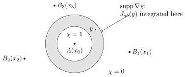
|
Figure 12. The shell flux of Definition 6.8. The cutoff \(\chi\) equals one near the insertion \(A (x_0)\) and vanishes near the spectators \(B_i (x_i)\); the current is integrated against \(\nabla \chi\) on the shaded annulus. Conservation makes the flux independent of \(\chi\), so the annulus may shrink towards \(x_0\) or grow until it meets a spectator. It says nothing about flux through large spheres. The vanishing of the total angular flux at infinity is proved separately: on coordinate lines in Lemma 16.15, and for all configurations in Lemma 16.17. |
The sign convention can be seen in one free example (Figure 12).
By Lemma 16.1(iv), \(S^{\text{Max}}_2 (\mathcal{O}_{F^2}
(x), \mathcal{O}_{F^2} (y)) = c |x - y|^{-
8}\) with \(c = 3
d_{\mathfrak{g}} / \pi^4\). The translation shell Ward identity
Replacing \(T^{\text{Max}}\) by \(\lambda T^{\text{Max}}\) multiplies this flux by \(\lambda\), so the requirement that the flux be the derivative fixes both the normalization and the sign of the stress tensor. This is a free-field calculation; nothing is asserted here about the form of interacting correlations.
The next lemmas concern only the invariant polynomial algebra of Definition 6.3, realized by the Taylor sections of Lemma 10.2. A curvature jet of order \(j\) has weight \(j + 2\). Let \(\mathfrak{P}\) be the complex polynomial algebra on all on-shell jets, \(\mathfrak{P}_{\leqslant j}\) its subalgebra using orders at most \(j\), and \(\mathfrak{P}^G\) the invariant subalgebra. The invariant polynomials of weight at most \(d\) identify with \(M_d^{\text{Max}}\). For a spectator degree \(d\) put
with every polynomial Wick ordered at its own site. The degree of \(P\) is unrestricted. The next result says that spectators of one bounded degree detect every invariant polynomial, however high its jet order.
The proof has two stages. At a fixed jet order, finite generation and reflected positivity give a bound on the spectator degree. To make the bound independent of the jet order, a quadratic spectator isolates a highest-order jet derivative of \(P\) by its harmonic pole, and induction on weight removes that jet order.
The extraction rests on the difference between a single harmonic pole and a product of poles. In four dimensions \(K (z) = \partial_1 \partial_2 |z|^{- 2} = 8 z_1 z_2 |z|^{- 6}\) is harmonic and homogeneous of degree \(- 4\); multiplication by \(|z|^4\) leaves \(8 z_1 z_2 |z|^{- 2}\), which is not analytic at zero, and only \(|z|^6\) clears it. The product of two poles \(|z|^{- 2} \cdot |z|^{- 2} = |z|^{- 4}\) has the same degree but is already cleared by \(|z|^4\). In general a product of poles of orders \(r_1, r_2 \geqslant 2\) is cleared by \(|z|^{2 (r_1 + r_2 - 2)}\), while a harmonic pole of order \(r_1 + r_2\) needs \(|z|^{2 (r_1 + r_2 - 1)}\).
Proof of Lemma 16.2. Step 1: bounded jet order. Fix \(j\). The algebra \(\mathfrak{P}_{\leqslant j}\) is a polynomial algebra on finitely many variables, hence Noetherian by the Hilbert basis theorem [33, Lemma 10.31.1]. Its ideal generated by invariant polynomials of positive ordinary degree therefore has finitely many invariant, ordinary-homogeneous generators \(f_{\alpha}\). Every invariant ordinary-homogeneous polynomial is a sum of products of invariant homogeneous polynomials of weight at most some \(b_j\): write \(P = \sum a_{\alpha} f_{\alpha}\), keep only terms of total degree \(\deg P\), and replace \(a_{\alpha}\) by its gauge average, whose degree is smaller; induction on the degree concludes.
Spectators of degree \(b_j\) detect: \(\mathfrak{N}_{b_j} \cap \mathfrak{P}^G \cap \mathfrak{P}_{\leqslant j} = \{0\}\). Otherwise take its lowest nonzero ordinary-homogeneous part \(P_r\) and split a product of homogeneous factors of total ordinary degree \(r\) into distinct nearby spectator sites. Every leg of \(P\) must pair with a spectator leg, so terms with internal spectator contractions, or with higher-degree parts of \(P\), vanish. As the spectator sites coalesce, Wick's rule gives the two-site pairing of \(P_r\) with their ordinary product. Each factor has weight at most \(b_j\), so for \(P \in \mathfrak{N}_{b_j}\) this limit is zero. Choose the product sum to be the reflection of \(\overline{P_r}\); Lemma 16.1(ii) makes this pairing strictly positive, a contradiction.
Step 2: pole extraction. Put \(g = d_{\mathfrak{g}}\) and choose \(d_0 \geqslant \max \{b_g, 2 g + 5\}\). In a real colour basis write \(X_{j, \alpha} (p)\) for the jet coordinate tested by a scalar order-\(j\) probe \(p\). For scalar probes \(p, q\) of orders \(k, l\), the invariant quadratic \(\sum_{\alpha} : X_{k, \alpha} (p) X_{l, \alpha} (q)\): has weight \(k + l + 4\). Its collision with a polynomial using jets through order \(j\) has, in the coefficient where just the order-\(k\) leg contracts at order \(j\), the polynomial
| \(\displaystyle \sum_{\alpha} X_{l, \alpha} (q) \sum_{\mu} C_{k, j} (p, e_{\mu} ; z) \frac{\partial P}{\partial X_{j, \alpha} (e_{\mu})},\) | (16.8) |
where \((e_{\mu})\) is a basis of order-\(j\) probes and \(C_{k, j}\) their differentiated curvature covariance.
Claim. If \(P \in \mathfrak{N}_{d_0}\), \(l < k\) and \(k + l +
4 \leqslant d_0\), then
Indeed \(\Delta (|z|^{2 s} K) = 4 s (s + 1 - r) |z|^{2 s - 2} K\) in
four dimensions; successive Laplacians show that \(K\) extends
analytically, and negative homogeneity makes it zero. Expand the
collision through an order exceeding \(8 + k + l + 2 j\). Since its
correlation with the quadratic test and further bounded-degree
spectators vanishes identically, comparing successive radial
homogeneities makes the order-\(r\) harmonic pole zero, so
Step 3: induction on weight. Take \(k = g + 1\) and \(l = 0,
\ldots, g - 1\). For each \(l\) choose a probe \(q_l\) and a jet value
\(v_l\) with \(q_l (v_l) = 1\). The matrix \((X_{l, \alpha} (q_l))_{l,
\alpha}\) has nonzero polynomial determinant: assigning \(v_l\) to
colour \(l\) and zero to the other colours in order \(l\) makes it the
identity. For \(j > g\) the polynomial
Let \(\mathcal{C}_d\) be the real space of complex linear tuples \(\textsf{X}_a : M_d^{\text{Max}} \to M_{d + 1}^{\text{Max}}\) that commute with conjugation, kill the unit, are vector-covariant under \(H_4\), and send \(M_e^{\text{Max}}\) into \(M_{e + 1}^{\text{Max}}\) for \(e \leqslant d\). For \(\textsf{X} \in \mathcal{C}_d\) the Ward sum is
Finitely many tests on lines determine its kernel.
Lemma
Proof. Take \(d \geqslant d_0\) from Lemma 16.2. Suppose all the stated jets of the Ward sums of \(\textsf{X}\) vanish.
Step 1: continuation off the lines. Free correlations are real
analytic off the diagonals by
Step 2: weight four. Let \(\textsf{J}_j\) be the scalar on-shell order-\(j\) jet space. For \(p \in \textsf{J}_0^{\ast}\) put \(U (p) = \sum_{\alpha} : X_{0, \alpha} (p)^2\):. Simplicity, the filtration and inversion parity force \(\textsf{X}_b U (p)\) to be a colour contraction of one order-zero and one order-one jet, represented by a linear map \(A_p : \textsf{J}_0 \to \textsf{J}_1^{\ast}\). In the Ward identity of \(U (p), U (q), U (w)\) let the first two points coalesce along \(tu\) and multiply by \(t^5\). The term with \(\textsf{X}_b\) at the distant point tends to zero, and the two remaining triangular Wick contractions give, for every \(X \in \textsf{J}_0\) and with \(C_{1, 0}\) taken in one colour,
Arbitrary \(X\) are reached by choosing the distant probe \(w\) through
the invertible order-zero covariance
Calculation of \(f_b\). Write \(e^{ij}\) for the curvature
coordinate and \(\partial_h e^{ij}\) for its first jet. For \(f_1
e^{12}\), sign parity permits only \(\partial_1 e^{12}, \partial_3
e^{23}, \partial_4 e^{24}\); interchange of axes \(3, 4\) and \(\sum_i
\partial_i e^{i 2} = 0\) reduce their span to \(\mathbb{R} \partial_1
e^{12}\). For \(f_1 e^{23}\) the candidates \(\partial_1 e^{23},
\partial_2 e^{13}, \partial_3 e^{12}\) reduce, by antisymmetry in axes
\(2, 3\) and Bianchi, to \(\mathbb{R} \partial_1 e^{23}\). Permutations
leave two constants, which agree because \(C_{1, 0} (\partial_1 e^{12},
e^{23} ; e_1 + e_3) = - 1 / (2 \pi^2) \ne 0\) by
Step 3: higher weights. Set \(\textsf{X}^{\circ}_b =
\textsf{X}_b - c \hspace{0.17em}
\partial^{\text{Max}}_b\). Translation
invariance makes its Ward sums zero, and it kills every free stress
component. Insert into such a sum a free stress shell for the dilation
field \(v (y) = y - x_0\), surrounding only the distinguished point. The
term where \(\textsf{X}^{\circ}_b\) acts on the stress is zero. The
other shell terms are given by the polarized calculation in Lemma 16.1, now with this \(v\); the extra derivative of \(v\)
contracts with the trace of the free stress, which is zero by
Step 4: finite selection. Conversely translation invariance annihilates every test on \(\partial^{\text{Max}}\). The real space \(\mathcal{C}_d\) is finite-dimensional; successively choose a test nonzero on the current kernel modulo this line. Each choice lowers its dimension, so finitely many tests have precisely the asserted kernel.\(\Box\)
The internal tests rest on one elementary fact about the plane generators \(K_{ab} = E_{ba} - E_{ab}\) of \(\mathfrak{so} (4)\). Call a coordinate quarter turn the rotation \(e_a \mapsto e_b\), \(e_b \mapsto - e_a\) in one coordinate plane.
Lemma
Proof. The quarter turns generate the determinant-one signed permutations: they project onto the transpositions of \(S_4\), and squares of quarter turns give the diagonal sign changes with two minus signs. Conjugation by a diagonal sign matrix \(s\) multiplies \(K_{ab}\) by \(s_a s_b\); conjugation by a permutation matrix permutes the planes. Overlapping planes: \(s = \text{diag} (1, 1, - 1, - 1)\) fixes \(K_{12}\) and reverses the sign of \(K_{13}\), so \(\beta (K_{12}, K_{13}) = - \beta (K_{12}, K_{13}) = 0\). Disjoint planes: the even permutation \((13) (24)\) interchanges \(K_{12}\) and \(K_{34}\), so \(\beta (K_{12}, K_{34}) = \beta (K_{34}, K_{12}) = - \beta (K_{12}, K_{34}) = 0\). Every pair of distinct planes is carried to one of these two pairs by a signed permutation of determinant one, and \(\beta (K, K) = 0\); bilinearity gives \(\beta = 0\).\(\Box\)
Let \(\mathcal{B}_d\) consist of alternating real-bilinear families \(\Delta : \mathfrak{so} (4)^2 \to \text{End}_{\mathbb{C}} M_d^{\text{Max}}\) which commute with conjugation, kill the unit, preserve every lower-degree subspace, and satisfy
The next result removes the defect in the rotation commutator.
Lemma
| \(\displaystyle \sum_i S_n^{\text{Max}} (u_1, \ldots, \Delta (K, L) u_i, \ldots, u_n ; x), \qquad u_i \in M_d^{\text{Max}}, \quad x \in \text{Conf}_n,\) | (16.10) |
separate \(\mathcal{B}_d\).
Proof. Suppose all these sums vanish and fix \(\textsf{Z} = \Delta (K, L)\). On the weight-four space let \(b_x (u, v) = S_2^{\text{Max}} (u, v ; x, 0)\). The order-zero Kelvin formula and Wick's rule give \(b_x (u, v) = b_y (R^{\text{Max}} (\mathcal{R}_y \mathcal{R}_x) u, v)\) for \(|x| = |y| \ne 0\). Both \(\textsf{Z}\) and the orthogonal action preserve this space. Applying \(b_x (\textsf{Z} u, v) + b_x (u, \textsf{Z} v) = 0\) at \(x\) and \(y\), and nondegeneracy of \(b_y\), shows that \(\textsf{Z}\) commutes with \(R^{\text{Max}} (\mathcal{R}_y \mathcal{R}_x)\), in particular with every coordinate quarter turn. With the signed covariance of \(\Delta\), the function \((K, L) \mapsto \Delta (K, L) u\) satisfies the hypothesis of Lemma 16.4 for each weight-four \(u\), so \(\textsf{Z}\) vanishes on weight four, including the stress.
Insert a free angular stress shell around the distinguished point only, as in Step 3 of the proof of Lemma 16.3. Subtracting the Ward sum with the angularly differentiated label gives \([\textsf{L}^{\text{Max}} (M), \textsf{Z}] u \in \mathfrak{N}_d\). This polynomial has weight at most \(d\), so Lemma 16.1(ii) makes it zero. Hence \(\textsf{Z}\) commutes with all infinitesimal rotations, and differentiating \(e^{t \textsf{L} (M)} \textsf{Z} - \textsf{Z} e^{t \textsf{L} (M)}\) gives commutation with coordinate quarter turns in every degree. Lemma 16.4 again gives \(\Delta = 0\). Finite-dimensionality selects a finite separating subfamily by successively reducing the common kernel.\(\Box\)
The insertions are those of Definition 2.8, with
coefficient polynomials from Definition 10.1 and Lemma 10.2. The inverse coefficient estimate of Lemma 14.6
inverts the marked coefficient map; the corrected sources and normalized
integral of Lemmas 14.24 and 14.25 bound the
remainders; the uniform displacement estimate of Lemma 14.27
controls positions, with coordinate separations at least four times the
displacement margin. Chessboard seminorms are those of Definition 14.10. Cutoff limits are taken in the order
Fix arity and degree bounds \(n \geqslant 2, D \geqslant 1\) and \(R \geqslant 1\). A basis word is a list of members of fixed real bases of \(M_d^{\text{Max}}\), \(d \leqslant D\). Put
The comparison exponents \(\alpha_0, \alpha_1, \alpha_2 > 0\) and \(c < 0\) have the following roles: \(\alpha_0\) sets the comparison radius, \(\alpha_1\) the cells used for moment bounds, \(\alpha_2\) the smaller cells used for displacement bounds, and \(c\) the width of the excluded coordinate strips. They satisfy
| \(\displaystyle \alpha_1 + 6 < \alpha_0, \quad \alpha_2 + 5 < \alpha_0 + c, \quad (\alpha_0 - \alpha_1) Dn + c < 0, \quad (\alpha_0 - \alpha_2) Dn - \alpha_0 - c < 0.\) | (16.11) |
The first two inequalities place the chessboard cells; the last two make the excluded strips negligible. One explicit choice, with \(n_{\max} = \max (n, D)\), is \(\kappa_1 = 7 n_{\max} (n_{\max} + 2) + 1\), \(\kappa_2 = 6 + \kappa_1\), \(\alpha_0 = 17 + n_{\max} + \kappa_1 + \kappa_2 n_{\max} (n_{\max} + 2) + \kappa_2\), \(\alpha_1 = \alpha_0 - 7\), \(\alpha_2 = \alpha_0 - \kappa_2\) and \(c = - \kappa_1\). Write \(M_k = M^{\text{cut}}_k\) and set
where \(C \geqslant 1\) depends only on \(n, D, R\) and the construction and is fixed in the proof of Lemma 16.6. Thus \(r_k \mathfrak{s}_k = a_k\): the normalized grid is the physical construction grid. For an ordered limit point \(c_{k, d} : M_d^{\text{Max}} \to V_d\) of the lifts in Lemma 16.6, and the quotient \(\pi_d : V_d \to F_d\) of Definition 2.12, define the rescaled correlation
The following comparison uses one coefficient family for every word within the fixed bounds. Its constants may depend on these bounds, the word and the construction. The arity, degree and radius bounds are fixed first, then the level and the lifts; the estimates then hold for every basis word within these bounds.
Lemma
At fixed \(k\) the lifts are bounded on ordered tails.
The lifts are chosen so that the rescaled insertions have the free Wick
polynomials as Gaussian leading part
Proof. Step 1: lifts. Choose a real \(H_4\)-equivariant polynomial representative map \(\iota_d^{\text{free}}\) for the on-shell quotient, using the Taylor sections of Lemma 10.2 and averaging a real splitting over \(H_4\). Let \(\textsf{C}_{k, N, p, d}\) be the marked coefficient map from level \(k\) down to \(m_{\text{ref}} (d)\), after the Wick-ordering correction of Lemma 14.23. Write \(\delta_t^{\text{wt}}\) for multiplication of a weight-\(j\) monomial by \(t^j\); the factor-count scaling \(t^{\textsf{N}}\) is that of Definition 2.8. The Gaussian field divided by the small-field threshold has scale
since \(t_k = M_k / \sqrt{\hat{\beta}_k}\) is the small-field threshold of Part I and \(\beta_{N, p, k} \leqslant 2 \hat{\beta}_k\). Solve
| \(\displaystyle \textsf{C}_{k, N, p, d} \Lambda_{k, N, p, d} u =\mathfrak{t}_{k, N, p}^{- \textsf{N}} \delta_{M_k^{\alpha_0}}^{\text{wt}} \iota_d^{\text{free}} u.\) | (16.14) |
The solution exists and obeys
| \(\displaystyle |v|_1 \leqslant K_{k, d} a_k^d | \textsf{C}_{k, N, p, d} v|_1,\) | (16.15) |
with \(K_{k, d}\) independent of \(N, p\) at fixed \(k\). Indeed, apply the inverse estimate of Lemma 14.6 at each step \(m + 1 \to m\) from level \(k\) down to \(m_{\text{ref}} (d)\), and the coefficient comparison in the proof of Lemma 14.23, whose relative error is less than \(1 / 4\), so its inverse costs at most \(2\). One may take \(K_{k, d}\) to be twice the product of the finitely many column and block factors up to \(k\), enlarged by the fixed basis norms. The coefficient map is injective, hence invertible on its finite coefficient space, and its unit, conjugation and signed laws pass to the inverse. The bound on \(\mathfrak{t}^{- 1}\) bounds the right side at fixed \(k\), so the lifts are bounded on cutoff tails.
Step 2: subset recursion. Lemmas 14.23–14.25 hold for an arity bound \(n \geqslant 2\), at most \(n\)
marks per cell and any compact position set with positive point
separation; apply them to the interval
This subtracts the full continuum Gaussian moment on every subset of
slots; for exact continuum Gaussian variables its nonempty coefficients
have expectation zero, by induction on \(|I|\). The Wick-ordering
correction and
Step 3: chessboard seminorm of the remainders. The finite-set
clause of Lemma 14.2 gives arbitrarily late common terminal
levels \(k\) for the three exponents \(\alpha_0, \alpha_1, \alpha_2\).
Use the interval
The normalized positive integral costs, per cell, at most the stage
constant \(Q_{J_k}^{\text{cmp}}\) of
The smallness comes from the corrected density at large coupling: its source terms stay bounded at a growing mark weight, while the unmarked normalization grows more slowly than that weight. The estimate concerns the complete reflected array, before absolute values are taken, and needs no independence of the insertions.
Step 4: comparison on the grid. Distinct coordinate differences
at normalized grid points are at least \(\mathfrak{s}_k\), so their
physical differences are at least \(a_k\). The reading map assigns the
corresponding level-\(k\) sites without rounding, and the interval
margin
Step 5: size and variation off the grid. At its own
normalization the singleton comparison gives a chessboard seminorm at
most \(1 + |S_1^{\text{Max}} (u) |\). For exponent \(\alpha_1\),
changing normalization to \(M_k^{\alpha_0}\) multiplies a weight-\(j\)
coefficient by \(M_k^{(\alpha_0 - \alpha_1) j}\), so the finite
coefficient sum bounds these seminorms by \(R^{\text{cell}}_k\) for
\(C\) large; exponent \(\alpha_2\) gives \(R^{\text{var}}_k\). Include
every reflected basis label and its complex conjugation in these maxima.
The two interval lengths of
| \(\displaystyle \frac{a_{w_b (k)}}{a_k} = L^{h_k (b) + v_k} \leqslant L^2 M_k^{b + 2} B_k^{10} \leqslant M_k^{b + 5} \qquad (b = \alpha_1, \alpha_2),\) | (16.17) |
after the stage entry, where \(L\) is fixed and \(B_k = M_k^{o (1)}\).
So the \(\alpha_1\) cell is at most \(a_k M_k^{\alpha_1 + 6} = o (r_k)\)
and the \(\alpha_2\) cell is \(o (r_k \delta_k)\) by
Step 6: limits. Take any ordered limit point of the bounded
lifts. Lemma 14.33 and
For the shell estimate take \(\varkappa \in \{0, 1\}\), \(A \in F_d\), \(B \in F_4\) and \(D = d + 1 - \varkappa\). The shell factor has scaling degree \(3 + \varkappa\): integration over four dimensions contributes four powers of the radius, the differentiated cutoff removes one, and the constant or linear vector field contributes \(\varkappa\). Since the two inserted fields have total degree \(d + 4\), the expected output degree is \((d + 4) - (3 + \varkappa) = D\). A grid test is a separated configuration \((0, x_i)\) on \(a_{j_0} \mathbb{Z}^4\) for some level \(j_0\), generic in each coordinate, with a fixed spectator list \(\boldsymbol{B}_i\). Its response functional and marked response are
Finite collections may use different grids, and the union of all these configurations is dense. The next lemma shows that every finite combination of tests annihilating \(F_D\) also annihilates the limiting shell response.
Lemma
Proof. The local sections of Lemma 10.2
and Lemmas 14.7–14.15 represent the
product of two nearby marked insertions by one marked insertion of
degree \(D\); Proposition 6.4 and Lemma 15.5
pass to the quotient. Put \(h = 3 + \varkappa\), so \(D + h = d + 4\).
Recall \(s_m = \log (a_m^{- 1})\) from
Step 1: two-mark representation. Fix a centered cell around the distinguished point, disjoint from all spectator stencils, and a finer stopping level \(k_0 \geqslant m_{\text{ref}} (D)\) at which its replicated source estimate applies. Choose levels \(j (m)\) with
they exist since \(s_{m + 1} / s_m \to 1\) (Lemma 14.2). At a grid point \(y \in a_{j (m)} \mathbb{Z}^4\) with \(\rho_m / 16 < |y| < 4 \rho_m\), choose representatives \(a \in V_d, b \in V_4\) of \(A, B\), block their two marked insertions at \(y, 0\) together, and retain the Taylor terms of weight at most \(D\). Their coefficient vector \(c_{N, p} (y) \in V_D\) is chosen by inverting the marked coefficient map. The exact difference is
Let \(u_{m, 1}, u_{m, 2}\) be the available mark weights of the
degree-\(d\) and rescaled degree-four marks at level \(j (m)\). The
one-mark bounds, including \(\rho_m^h\), give \(\log u_{m, 1} = (- dt +
o (1)) s_m\) and \(\log u_{m, 2} = (- 4 t + h + o (1)) s_m\); support
weights, coefficient columns and threshold powers have logarithm \(o
(s_m)\) by
| \(\displaystyle \log v_m = [- D - (d + 12) (t - 1) + o (1)] s_m, \qquad e_m \leqslant \exp \{[(d + 12) (t - 1) + o (1)] s_m \} .\) | (16.19) |
Indeed the transported exponents sum to \(- (d + 4) t + h + 8 (1 - t) =
- D - (d + 12) (t - 1)\), and Taylor extraction costs the reciprocal
joint weight times \(a_{m + 1}^D\), which cancels the \(D\) term. This
is the two-mark use of the source representation
Step 2: backward matching. Apply
which eventually fits every fixed source allowance at \(k_0\). The
residual-source estimate
Step 3: cancellation at grid points. Pass to an ordered limit
point \(c (y)\) and project it to \(F_D\). The chessboard inequality
with the same coefficient vector for every spectator. Multiplication by \(g_i\) and summation cancel the response term, so \(f_m (y) = \sum_i g_i \rho_m^h \mathfrak{h}_i (y)\) is \(O (c_m^{- 1})\) at all grid points of the enlarged annulus whose four coordinates are nonzero.
Step 4: interpolation across coordinate planes. For a
derivative order \(q\), Proposition 6.4 replaces the moving
label by one of degree \(4 + q\). The centered and reflected bounds of
Lemmas 14.15 and 14.14, with
| \(\displaystyle | \partial_a^q f_m (y) | \leqslant \exp [(q + C_0 + o (1)) s_m] \qquad (\rho_m / 16 < |y| < 4 \rho_m),\) | (16.20) |
with \(C_0\) independent of \(q\). Choose \(q\) with \(q (t - 1) > C_0\); since \(a_{j (m)} = \exp [- (t + o (1)) s_m]\), the \(q\)th derivatives along grid-sized segments tend to zero. On each coordinate segment of length \(4 (2^q + 2) a_{j (m)}\) choose \(q\) grid nodes with nonzero coordinates, mutually separated by at least \(a_{j (m)}\). Lagrange interpolation gives \(|g| \leqslant C_q (\max_{\text{nodes}} |g| + a_{j (m)}^q \sup | \partial^q g|)\) on the segment, with \(C_q\) independent of \(m\). Apply it to Re\(\hspace{0.17em} f_m\) and Im\(\hspace{0.17em} f_m\) in each of the four axes; the segments stay in the enlarged annulus since \(4 (2^q + 2) a_{j (m)} = o (\rho_m)\). Four successive interpolations give \(\sup_{\rho_m / 4 \leqslant |y| \leqslant 2 \rho_m} |f_m (y) | \to 0\). Select a decreasing subsequence of \(\rho_m\); it depends on the fixed tests and \(g\), as allowed.\(\Box\)
The next lemma converts Lemma 16.6 into the comparison of Part I, measured uniformly over the supremum-norm unit ball of tests. No volume refinement is needed.
Lemma
Proof. Lemma 16.6 supplies the three estimates, Lemma 16.1 the free modulus of continuity and the free separating tests, and Proposition 6.4 the dimension bound. The set \(K_{R, m} \setminus E_{8 \delta_k}\) lies in finitely many strips about coordinate coincidence hyperplanes and has volume at most \(C_{m, R} \delta_k\); its contribution to a tested difference is at most \(C_{m, R} \|f\|_{\infty} ((R^{\text{cell}}_k)^m +\|S^{\text{Max}}_m \|_{K_{R, m}}) \delta_k\). Outside these strips, rounding to the grid moves a point by at most \(4 m\mathfrak{s}_k \leqslant \delta_k\), so the segment stays in \(K_{2 R, m} \cap E_{4 \delta_k}\). The mean value bound and the free modulus of continuity \(\varpi\) give total tested error at most
Every term tends to zero by the strict inequalities
At a fixed comparison level the lifts are bounded in a
finite-dimensional space. Take an ordered limit point and project to
\(F_d\); ordered convergence holds also for convergent coefficients, by
multilinearity. This proves
Choose successively arity, degree and radius bounds tending to infinity,
tolerances tending to zero, and strictly decreasing radii tending to
zero; this is possible because \(\log M_k = o (\log a_k^{- 1})\) by
| \(\displaystyle \tilde{U}_{k, 0} = U_{k, 0}, \qquad \tilde{U}_{k, d + 1} = \jmath_{d, d + 1} \tilde{U}_{k, d} L_d + U_{k, d + 1} (I - i_d L_d) .\) | (16.22) |
The first summand is exact on included fields and the second agrees with \(U_{k, d + 1}\) on a complement; since free and interacting inclusions preserve correlations, the comparison is preserved, as are reality and signed covariance, and the degree-zero unit gives all units. Strict free positivity supplies finitely many separating tested correlations in each degree; their matrices converge, so a nonzero full-rank minor makes \(\tilde{U}_{k, d}\) eventually injective, and Proposition 6.4 makes it an isomorphism. Fill the finitely many earlier indices in each degree with any of these isomorphisms.\(\Box\)
Proof of Proposition 6.7. By the equivalence after Proposition 6.7, uniform tested convergence on each compact set is local \(L^1\) convergence; Lemma 16.8 gives it for one stable sequence.\(\Box\)
The comparison upgrades to smooth convergence, which the identification of the current needs.
Corollary
| \(\displaystyle \textsf{d}_{k, a} = r_k (\textsf{U}_{k, d + 1}^{\text{sc}})^{- 1} \partial_a \textsf{U}_{k, d}^{\text{sc}} \longrightarrow \partial_a^{\text{Max}}\) | (16.23) |
in operator norm, and, whenever \(u_{k, i} \to u_i\),
Proof. Choose finitely many tested free
responses injective on \(M_{d + 1}^{\text{Max}}\); their interacting
matrices converge to this injective matrix by Lemma 16.8.
Testing \(\textsf{d}_{k, a} u\) gives, by integration by parts, minus
the correlation tested against \(\partial_{x_0^a} f\), which converges
to the test of \(\partial_a^{\text{Max}} u\). An injective finite matrix
has a bounded left inverse on all small perturbations, proving
The chain rule and
The rank calculation
Lemma
componentwise.
Proof. Transport a free tensor by
\(\textsf{U}_{k, 4}^{\text{sc}}\) and subtract its mixed one-point value
times the unit. On centered tensors this is a real isomorphism \(C_k\);
the inverse transports back and subtracts the free expectation, and unit
preservation makes the two composites identities. Let \(V_k\) be
transport by \(\textsf{U}_{k, 5}^{\text{sc}}\) on real covariant
vectors. By
the centering term disappearing since derivatives kill the unit.
Composition with a right inverse of free divergence tends to the
identity, so mixed divergence is onto. The domain and target have
dimensions three and two by these isomorphisms and
Choose a nonzero \(B\) on this line and set \(c_k = \|(\textsf{U}_{k,
4}^{\text{sc}})^{- 1} (r_k^4 B)\| / \|T^{\text{Max}}
\|\), with norms on
whole tensors. The normalized preimages have a convergent subsequence on
this sphere. Stability preserves symmetry, reality and signed
tensoriality;
Lemma 16.7 now applies to each component of the current, and the resulting fields represent both fluxes of Definition 6.8. The proof combines it with finite-dimensional duality, conservation, translation covariance and continuity of separated responses.
Lemma
Proof. Use a constant Killing field \(v\) (\(\varkappa = 0\)) or \(v (y) = Ky\) (\(\varkappa = 1\)). Independence of the shell cutoff follows by integration by parts: the divergence vanishes, and \(\sum_{a, b} (\partial_a v_b) J_{ab} = 0\) by symmetry.
Fix finitely many grid response tests \(\textsf{r}_i\) and coefficients \(g_i\) annihilating \(F_D\), \(D = d + 1 - \varkappa\). Shrink a common shell cutoff to \(\chi (y / \rho_l)\), with \(\chi = 1\) near zero and \(\nabla \chi\) supported in \(1 / 2 \leqslant |y| \leqslant 1\). Changing variables gives the sum of their fluxes as
which is independent of \(l\) and tends to zero by
Choose a finite separating family of grid tests; it exists because the common kernel of all separated responses is zero, grid configurations are dense, and responses are continuous. A field matching this family is unique, and adjoining any further grid test, the same field matches it. Continuity of the responses and of shell integrals, with the cutoff fixed locally, extends the identity to all separated configurations with distinguished point zero; translation covariance moves that point to arbitrary \(x_0\). Linearity of the integral and injectivity of responses give complex linearity in \(A\) and real linearity in \(K\). Taking \(v = e_b\) and \(v = K (\cdot - x_0)\) gives the two raw shell identities.\(\Box\)
Coordinate reflection positivity alone gives a reflection Hilbert space for each coordinate axis. This subsection constructs these spaces, bounds the slab insertion operators, and bounds the low-energy spectral mass of collinear words of mixed reflection parity and of the components of a conserved tensor. Section 16.5 uses these bounds to remove the boundary at infinity before continuous rotations are known. Nothing here uses rotations or Sections 16.1–16.3: the inputs are E1–E7, Proposition 6.4 and Lemmas 15.6–15.7.
A word is \(w = \prod_{i = 1}^n A_i (x_i)\) with distinct points, and \(\tau_z w = \prod_i A_i (x_i + z)\). Fix a norm \(\| \cdot \|_{V_d}\) on each coefficient space; insertion-label bounds refer to representatives in the spaces \(V_d\) of Definition 2.8, and the resulting operators depend only on their classes in \(F_d\). Write \(w^{\ast}\) for the word with reversed order and conjugated labels, extended antilinearly to word combinations, \(\vartheta\) for linear time reflection, acting on labels through the hypercubic action of \(\textsf{s}_4^{\text{refl}}\), and \(\theta w = \vartheta w^{\ast}\); thus \(\theta\) is the antilinear reflection in the form of Definition 6.5. The insertion rule and buffer are those preceding Lemma 15.7: \(A_w v = w \hspace{0.17em} \tau_{he_4} v\), and an \(r\)-buffered word in width \(h\) has mutual sup-distance at least \(r\) and times in \([r, h - r]\). Write \(\partial_{i, a} w\) for the word with \(A_i\) replaced by \(\partial_a A_i\).
Repeated reflected insertions bound the operator that inserts a word into a time slab. Taking arbitrarily high powers removes the dependence of the bound on the exterior vector.
Lemma
with derivatives in operator norm; the empty word gives \(e^{- hH_4^{\text{OS}}}\).
Proof. Replace \(R\) by \(\max (1, R)\). The heat semigroup. On the span of positive words, \(\| \tau_{te_4} v\|^2 = \langle v, \tau_{2 te_4} v \rangle \leqslant \|v\| \hspace{0.17em} \| \tau_{2 te_4} v\|\). E7 bounds the separated orbit, so iteration gives \(\| \tau_{te_4} v\| \leqslant \|v\|\) and null vectors are preserved. Translation invariance gives symmetry and commuting unitary spatial translations; Gram continuity gives strong continuity. Since \(e^{- H} \psi = 0\) implies \(e^{- 2^{- j} H} \psi = 0\), strong continuity excludes spectral mass at zero of the heat operator. Spectral calculus [19, Theorem 2.5.1 and Proposition 4.2.3] defines \(H_4^{\text{OS}} = \int_{(0, 1]} - \log v \hspace{0.17em} dP (v)\) from the spectral measure \(P\) of the time-one heat operator; positive roots and continuity give \(e^{- tH_4^{\text{OS}}} \to P_4^0\) strongly.
The power argument. For a nonempty word, Lemma 15.7 supplies a width \(s\) and \(D = C_0^n (n / r)^{Qn}\). On the word span put \(A = A_w\), \(B = A_{w^{\dagger}}\) with \(w^{\dagger} = \tau_{se_4} \theta w\), and \(T = BA\). The OS form gives \(\langle Av, u \rangle = \langle v, Bu \rangle\), and Lemma 15.7 gives \(\|T^j v\| \leqslant K_v D^{2 j}\). Set
Symmetry of \(T\) gives \(d_j^2 \leqslant \|v\| d_{2 j}\), hence \(M_v^2 \leqslant \|v\| M_v\) and \(M_v \leqslant \|v\|\). In particular \(\|Av\|^2 = \langle v, Tv \rangle \leqslant \|v\| \hspace{0.17em} \|Tv\| \leqslant D^2 \|v\|^2\). The bound is independent of \(K_v\), and density gives the unique bounded extension. Right multiplication by \(e^{- (h - s) H_4^{\text{OS}}}\) gives the required width.
Identities. Positive-word matrix entries prove
With \(e_{\mu}\) as time, the same construction gives \(\mathcal{H}_{\mu}^{\text{OS}}\), \(e^{- tH_{\mu}^{\text{OS}}}\) and commuting transverse translations \(\textsf{T}_{\perp} (y)\), \(y^{\mu} = 0\), using only coordinate reflection positivity and signed permutations. Their joint projection-valued measure \(P_{\mu}\) lives on \([0, \infty) \times \mathbb{R}^3\), with variables \((E, p)\): apply Gelfand theory to the commutative unital C\(\ast\)-algebra generated by \(e^{- H_{\mu}^{\text{OS}}}\) and the translation representation of \(C_0 (\mathbb{R}^3)\) [19, Theorems 2.4.1, 3.7.11, equation (3.89) and Proposition 4.2.3], then take the logarithm of the heat coordinate. For a word combination \(U\), let \(v_{\mu, u} (U)\) be its OS vector translated by \(ue_{\mu}\) into positive times, and undo the damping by
| \(\displaystyle d \nu_{\mu}^U (E, p) = e^{2 uE} \hspace{0.17em} d \langle v_{\mu, u} (U), P_{\mu} (E, p) v_{\mu, u} (U) \rangle .\) | (16.27) |
This measure is independent of \(u\) and finite on \(E \leqslant M\); point-field measures may have infinite total mass before damping. Polarize to \(\nu_{\mu}^{UV}\) on integrable tests. For nonnegative integrable \(g_1, g_2\), spectral Cauchy–Schwarz gives
If \(\vartheta_j U = \varepsilon_j U\) with \(\varepsilon_j \in \{1, - 1\}\), then, for \(x^{\mu} = 0\) and \(t\) separating the words,
Both point fields and collinear words are represented.
Opposite reflection signs compare coordinate spectra. Fix a set of axes \(\mathcal{A} \subset \{1, 2, 3, 4\}\) and a finite word combination \(U\) whose offsets have zero coordinates in \(\mathcal{A}\), with \(\vartheta_j U = \varepsilon_j U\) for \(j \in \mathcal{A}\), and assume that both signs occur. For even nonnegative \(f_j \in C_c^{\infty} (\mathbb{R})\) set \(f_{j, v} (p) = v^{- 1} f_j (p / v)\). Throughout, \(\lambda\) ranges over \(e^{\mathbb{N}}\).
Lemma
Constants may depend on \(U, \mathcal{A}, q, \beta, f, \delta\).
Tested against a product of even profiles, the reflected correlation of
\(U\) has a positive spectral representation in each time axis \(i \in
\mathcal{A}\), with sign \(\varepsilon_i\). For two axes of opposite
parity, these representations of the same number differ by a sign; after
the annular corrections below, this gives the transfer inequality
Proof. Moments. For a placement of margin \(r > 0\), E7 bounds the \(2 m\)th transverse derivative of the reflected-pair correlation by \(Cr^{- D}\). Its centered difference has spectral integrand \([2 \sin (tp_j / 2) / t]^{2 m} e^{- 2 uE}\), and the integral remainder formula and Fatou give
| \(\displaystyle \int e^{- 2 uE} |p_j |^{2 m} \hspace{0.17em} d \nu_{\mu}^U \leqslant Cr^{- D} .\) | (16.29) |
Extra heat supplies energy powers, so for every damping \(u\) as in
| \(\displaystyle \int e^{- 2 uE} (1 + E + |p|)^m \hspace{0.17em} d \nu_{\mu}^U < \infty \hspace{0.17em} .\) | (16.30) |
For offsets perpendicular to \(\mu\) take \(u = t / 2\), \(r \asymp t\); integrating \(Ct^{- D}\) against \(t^D \hspace{0.17em} dt\) on \((0, 1)\) gives, after enlarging \(D\), \(\int (1 + E)^{- D} |p_j |^{2 m} \hspace{0.17em} d \nu_{\mu}^U < \infty\).
Annular correction. Choose even \(\sigma \geqslant 0\) of integral one supported in \(1 \leqslant |v| \leqslant 2\). Let \(L_j\), \(0 \leqslant j < m\), be the Lagrange polynomials of degree \(m - 1\) with \(L_j ((i + 2)^2) = \delta_{ij}\). For radius \(\varrho > 0\) define
Since \(\sum_j L_j (x) (j + 2)^{2 i} = x^i\) for \(i < m\), the residual \(f -\mathcal{C}_{m, \varrho} f\) has vanishing moments \(\int p^{2 i} (\cdot) \hspace{0.17em} dp\) for \(i < m\), hence \(2 m\) vanishing moments when \(f\) is even; the correction is an annular profile whose coefficients contain \(\varrho^{- 2 r}\). Put \(\text{Lap} \hspace{0.17em} f (E) = \int e^{- E |t|} \hat{f}_+ (t) \hspace{0.17em} dt\). Interpolating \((p^2 + E^2)^{- 1}\) gives the residual response
Its value at \(E = 0\) is \(2 \pi f (0)\), and for \(f \geqslant 0\) supported in \([- \varrho, \varrho]\) all factors lie in \([0, 1]\). Let \(f \geqslant 0\) be even, supported in \([- 1, 1]\) and equal to one on \([- \tfrac{1}{2}, \tfrac{1}{2}]\), and let \(0 < v \leqslant 1 \leqslant \varrho\). Then
with \(C = C (m, D, \|f\|_{L^1})\): the upper bounds follow from \(2 E \int (p^2 + E^2)^{- 1} dp = 2 \pi\) and from bounding the product by \(\prod_j (2 \varrho (j + 2) / E)^2\); for the lower bound the product is at least \(2^{- m} (1 + E)^{- 2 m}\) for \(|p| \leqslant v\), and one integrates over \(0 < p < vE / (2 (E + v))\). With the moment bound, for \(\varrho \geqslant 1\), \(\text{supp} \hspace{0.17em} f_v \subset [- \varrho, \varrho]\) and \(m \geqslant D / 2\) chosen after the moment exponent \(D\),
| \(\displaystyle \int \mathcal{R}_{m, \varrho} f_v (E) |p_j |^{2 r} \hspace{0.17em} d \nu_{\mu}^U \leqslant C (v^{- 1} + \varrho^D) .\) | (16.32) |
Transfer between two axes. For \(i, j \in \mathcal{A}\) write \(\text{Resp}_i (g) = \int \text{Lap} \hspace{0.17em} g_i (E) \prod_{k \in \mathcal{A} \setminus \{i\}} g_k (p_k) \hspace{0.17em} d \nu_i^U\). For \(\mathcal{A}\) containing all axes, the same product test gives
since \(\int e^{ipx} \hat{g}_+ (x) \hspace{0.17em} dx = 2 \pi g (p)\)
for even profiles, while the time integral is \(\text{Lap}
\hspace{0.17em} g (E)\); both temporal profiles have the zero moments
required at collisions. For smaller \(\mathcal{A}\), put \(g_k (p) = h
(p / T)\) in omitted axes, with \(h \in C_c^{\infty} (\mathbb{R})\) even
and equal to one near zero, and let \(T \to \infty\) by
| \(\displaystyle \text{Resp}_i (g_i - a_i ; g_{\ne i}) \leqslant \text{Resp}_i (g_i - a_i ; g_j \mapsto a_j) + \text{Resp}_j (g_j - a_j ; g_i \mapsto a_i),\) | (16.33) |
after expanding the signed identity and discarding \(\text{Resp}_j (g_j - a_j ; g_{\ne j}) \geqslant 0\).
The walk. Choose a finite walk \(i_0, \ldots, i_L\) in \(\mathcal{A}\) with opposite signs at consecutive entries, \(i_0 = i\), every axis among \(i_0, \ldots, i_{L - 1}\), and \(i_L\) already visited; it exists because both signs occur (insert an axis of the opposite sign between two entries of the same sign). Put \(V_s = \{i_0, \ldots, i_{s - 1} \}\). Fix \(K \geqslant 0\) and \(\delta > 0\). The induction claim is that there is \(A_s > 0\) such that, for every fixed family of even nonnegative compactly supported profiles \(f_j\), all exponents with \(0 \leqslant \omega_j \leqslant A_s\) (\(j \in V_s\)) and \(- K \leqslant \omega_j \leqslant A_s\) (\(j \not\in V_s\)), every \(0 \leqslant \eta \leqslant A_s\) with \(\omega_{i_s} \leqslant \eta\), and \(R_0 \geqslant 1\) such that the profile in axis \(i_s\) is supported in \([- R_0 \lambda^{\eta}, R_0 \lambda^{\eta}]\), all large subtraction orders \(m\) satisfy
with \(C\) and the threshold in \(\lambda\) depending on the fixed data. Small positive exponents on unvisited axes permit later visits.
At \(s = L\) every width is at least one, so all transverse suprema are
bounded, and
| choice | depends on | |
| 1 | \(\alpha' = A_{s + 1}\) | the case \(s + 1\) of |
| 2 | \(r \in \mathbb{N}\) with \(2 r \alpha' > p_{\ast} + \max (K, \delta) + 1\) | \(\alpha', K, \delta, |\mathcal{A}|\) |
| 3 | moment exponent \(D\) of |
\(r, U\) |
| 4 | \(0 < A_s < \min (\alpha', \delta / (D + 1))\) | \(\alpha', \delta, D\) |
| 5 | subtraction orders \(m\) | \(D\) and the collision orders |
Correct the profile in axis \(i\) at radius \(R_0 \lambda^{\eta}\) and
the one in axis \(j\) at radius \(\lambda^{\alpha'}\). The correction in
\(i\) is bounded by a fixed even nonnegative annular profile of width
\(\lambda^{\eta}\), since its coefficients contain only factors
\(\lambda^{2 r' (\omega_i - \eta)} \leqslant 1\); so the second term of
Both residual responses are nonnegative, so
Conclusion. Apply the case \(s = 0\) with \(K \geqslant \max (-
q, \max_j (- \beta_j))\), \(\omega_i = q\), \(\omega_j = \beta_j\) for
\(j \ne i\), and \(\eta = 0\), the profile in axis \(i\) being the bump
of the lower response bound. On \(E \leqslant 1\) that bound makes the
stated integral at most \(c_m^{- 1}\) times the integral in
Fix \(a \ne b\) and a line axis \(l\). Set \(\omega_a = \omega_b = - 100\), \(\omega_l = - 150\) when \(l \not\in \{a, b\}\), and \(\omega_j = - 300\) for \(j \not\in \{a, b, l\}\). For a fixed even nonnegative \(\psi \in C_c^{\infty} (\mathbb{R})\) equal to one on \([- 1, 1]\) put
These are the scales of the box on which the vector field of Lemma 16.15 equals \(Ky\): \(|y_a |, |y_b | \leqslant \lambda^{100}\), \(|y_l | \leqslant \lambda^{150}\), \(|y_j | \leqslant \lambda^{300}\). Set \(B = 2^{- 4} \prod_j (1 + \varepsilon_j \vartheta_j) U\) for a word combination \(U\) with offsets on \(\mathbb{R}e_l\), with \(\varepsilon_a = \varepsilon_b = - 1\) and the other signs positive. Let \(J_{ij} \in F_4\) be real, symmetric, \(H_4\)-tensorial and conserved; no Ward normalization is assumed. The index \(J_{\mu b}\) in a measure denotes the one-point word \(J_{\mu b} (0)\). Consider also tests \(\Psi_{\lambda} (E, p)\) such that, for some fixed \(K\) and every \(L \geqslant 0\),
| \(\displaystyle | \Psi_{\lambda} (E, p) | \leqslant C_L \lambda^K e^{- \lambda^{- \omega_{\mu}} E} \prod_{j \ne \mu} (1 + \lambda^{- \omega_j} |p_j |)^{- L} \hspace{0.17em},\) | (16.34) |
and put \(X_{\lambda} = \{E > 1\} \cup \bigcup_{j \ne \mu} \{|p_j | > w_j \}\). The scaled Fourier–Laplace tests of Lemma 16.15, with fixed polynomial prefactors, have this bound. Constants below may depend on the fixed words, tensor, profiles and exponents.
Lemma
and \(I_{\mu} (J_{\mu \mu} ; 0) = O (\lambda^{900})\) and \(\int_{X_{\lambda}} \Psi_{\lambda} \hspace{0.17em} d \nu_{\mu}^{UV} = O_M (\lambda^{- M})\).
The sign estimates come from Lemma 16.13; the diagonal
estimate comes from conservation. Recall also
Proof. Sign estimates. In direction
\(l\), choose \(2 u\) separating the offsets and use \(R_v (E) = \int
e^{- E |t|} (1 - \chi (t)) \phi (vt) \hspace{0.17em} dt\), where \(0
\leqslant \chi \leqslant 1\) is compactly supported and equals one on
\([- 2 u, 2 u]\), and \(\phi = \widehat{(\sigma \ast \sigma)}_+
\geqslant 0\), \(\phi (0) = 1\). It satisfies \(C / (E + v) \leqslant
R_v (E) \leqslant C' v^{- 1} e^{- 2 uE}\) for \(E \leqslant 1\) and
small \(v\): integrate over \(R < t < R + c / (E + v)\) beyond
\(\text{supp} \hspace{0.17em} \chi\) for the lower bound, and drop \(1 -
\chi\) and scale for the upper. The removed profile has bounded
supremum, and
Diagonal tensor: moment-subtracted extension. Write \(C_{ab, cd} (x) = S (J_{ab} (0) J_{cd} (x))\), \(x \ne 0\). Choose \(D_{\text{col}}\) bounding the collision powers of these pairs and their first derivatives. For even \(\chi = 1\) near zero with compact support put \(\Pi_{D_{\text{col}}} f (t) = \chi (t) \sum_{r < D_{\text{col}}} f^{(r)} (0) t^r / r!\), and define
Taylor vanishing gives integrability, and a zero Taylor factor recovers the unsubtracted integral. Average under signed symmetries and pair exchange to obtain \(R\). Conservation makes \(\sum_i \partial_i R_{ib, cd}\) a jet at zero, and inversion \(x \mapsto - x\) makes \(R\) even, eliminating even divergence orders. To remove the linear orders, put \(\chi_0 (x) = \prod_j \chi (x_j)\) and \(q_{ab, cd} = \sum_i R_{ib, cd} (\partial_i (x_a \chi_0))\), and replace \(R\) by \(R_{ab, cd} - q_{ab, cd} \delta_0\); reflections kill coefficients unless indices occur in pairs, and permuting them gives the pair symmetries. Write \(\hat{R}_{ab, cd}\) for the Fourier transform of this corrected extension. Its divergence is the polynomial \(F_{b, cd} (p) = \sum_i p_i \hat{R}_{ib, cd} (p)\), with no terms of degree below three. Symmetry gives
and the same two contractions on the other index pair give
where multiplication by \(p_j\) acts on the test and \(D_1, D_2\) are polynomial remainders.
Diagonal tensor: annular bounds. On a fixed temporal annulus,
Lemma 16.13 and
Diagonal tensor: positivity. Put \(g_{v, r} (p) = v^{- 1} (p / v)^{- 2 r} \sigma (p / v)\), so \(p^2 g_{v, r + 1} = v^2 g_{v, r}\). Keep \(\mathcal{K}_{\lambda}\) fixed and set
Conservation gives \(c_{r + 1} (t) = t^2 c_r (t) + O_{\delta}
(\lambda^{\delta} W^2)\) for \(t = 1, 2\), \(r = 0, 1\). The correction
of \(g_{W, r} - g_{2 W, r}\) has zero zeroth moment and other even
moments \(O (W^2)\), so \(d_r = c_r (1) - c_r (2) + O_{\delta}
(\lambda^{\delta} W^2)\). Reflection positivity for \(J_{\mu \mu}\)
makes the spectral representation of \(\mathcal{Q}_0\) positive; on
corrected profiles it gives \(d_0 \geqslant 0\), \(d_1 \leqslant 0\),
\(d_2 \geqslant 0\), since multiplication by \(p_{\mu}^2\) becomes \(-
E^2\). Consequently \(4 d_0 = 5 d_1 - d_2 + O_{\delta} (\lambda^{\delta}
W^2)\) and \(d_0 = O_{\delta} (\lambda^{\delta} W^2)\). Subtracting
\((E^2 + 4 W^2 v^2)^{- 1}\) from \((E^2 + W^2 v^2)^{- 1}\) in
and multiplying by \(W^2 / c_m\) gives the third estimate.
Crude and far-region bounds. Finiteness of \(\nu_{\mu}^{J_{\mu
\mu}} (E \leqslant 1)\) and \(\|\mathcal{K}_{\lambda} \|_{\infty} = O
(\lambda^{897})\) give the crude bound. On \(E > 1\),
Write \(\boldsymbol{q}= (A_i (x_i))_i\) and define the angular sum
It is the total angular flux of the raw charges of Lemma 16.11.
Fix distinct axes \(a, b\), a line axis \(l\), and the exponents
\(\omega_j\), profile \(\psi\) and weights \(\mathcal{K}_{\lambda}\) of
Section 16.4. For a word \(B\) on \(\mathbb{R}e_l\)
projected to odd parity in \(a, b\) and even parity in the other axes,
Lemma 16.14 gives the sign estimates
The next lemma removes the angular boundary at infinity before continuous rotations are known. Its mechanism is as follows. The shell identities and conservation write the angular sum as the integral of the conserved tensor against the derivative of a vector field equal to \(Ky\) on a large box; the sum does not depend on the box, so it suffices that this integral tends to zero. No decay of correlations is assumed, so the smallness must come from positivity. After a translation the configuration lies on a line \(\mathbb{R}e_l\). A coordinate reflection in an axis other than \(l\) fixes every point of this line, and the reflection in \(l\) maps it to itself; so reflecting the integration variable replaces the spectator word by its parity projections, which are again combinations of words on the line, odd in \(a, b\) and even in the other axes. Such a word has positive spectral representations of opposite signs in two coordinate time axes, and Lemma 16.13 turns this into a bound on its low-energy spectral mass; the diagonal components of the tensor are controlled by conservation instead (Lemma 16.14). The box has the large anisotropic extents \(\lambda^{- \omega_j}\) of Section 16.4. In the terms that survive two exact cancellations, differentiating the cutoff in the time axis \(\mu\) leaves a profile of bounded \(L^1\) norm supported where \(|y_{\mu} | \geqslant \lambda^{- \omega_{\mu}}\), whose Laplace transform gains the factor \(\lambda^{\omega_{\mu}} / (E + \lambda^{\omega_{\mu}})\). On the momentum side the cutoff is concentrated where \(|p_j | \lesssim \lambda^{\omega_j}\); the windows \(|p_j | \leqslant w_j = \lambda^{1 + \omega_j}\) are wider by the factor \(\lambda\), so outside them every power of \(\lambda\) is gained. The exponents are chosen so that every term is \(O (\lambda^{- 101})\) before the prefactor \(\lambda^{100}\), the size of \(|Ky|\) on the box.
Lemma
Proof. It suffices to treat \(K = E_{ba} - E_{ab}\), \(a \ne b\), for which \((Ky)_b = y_a\), \((Ky)_a = - y_b\) and the other components vanish. Choose even \(\eta \in C_c^{\infty} (\mathbb{R})\) equal to one on \([- 1, 1]\) and put \(\ell (t) = t \eta (t)\). Set
The vector field \(V\) equals \(Ky\) on the box \(|y_a |, |y_b | \leqslant \lambda^{100}\), \(|y_l | \leqslant \lambda^{150}\), \(|y_j | \leqslant \lambda^{300}\), hence near every insertion for large \(\lambda\). Disjoint shell cutoffs, the raw shell identities of Lemma 16.11 and conservation give \(\text{Ang}_K = - \int \sum_{\mu, c} \partial_{\mu} V_c \hspace{0.17em} S (J_{\mu c} (y), \boldsymbol{q}) \hspace{0.17em} dy\).
Two exact cancellations. Only the columns \(c = a, b\) occur, since \(V_c = 0\) otherwise. Since \(\omega_a = \omega_b\), both \(\partial_a f_{ab}\) and \(\partial_b f_{ba}\) equal \(\prod_j \ell' (\lambda^{\omega_j} y_j)\), and \(J_{ab} = J_{ba}\); so the term \(\mu = a\) of the column \(b\) cancels the term \(\mu = b\) of the column \(a\):
These are identities for every \(\lambda\); no estimate enters them. The second sum is the first with \(a, b\) exchanged, and \(\omega_a = \omega_b\), so the bounds below for the first sum apply to it; this includes its diagonal component \(J_{aa}\). Since the angular sum is independent of \(\lambda\), it suffices to show that each term \(\mu \ne a\) of the first sum is \(O (\lambda^{- 101})\) before the prefactor \(\lambda^{100}\).
Spectral form of one term. Fix \(\mu \ne a\). Reflecting the
integration variable in each axis, including the tensor signs, replaces
the spectator word by its odd projection in \(a, b\) and its even
projections in the other axes; if the line axis is reflected, the
projection is a finite linear combination of collinear words. The term
becomes a pairing against the measure \(\nu_{\mu}^{B, J_{\mu b}}\), the
polarization of the coordinate spectral measures
Their product gives \(\lambda^3 \mathcal{K}_{\lambda}\). For an
off-diagonal component,
One term in detail. Take \(a = 1\), \(b = 2\), \(l = 3\), so \((\omega_1, \omega_2, \omega_3, \omega_4) = (- 100, - 100, - 150, - 300)\), and the term \(\mu = 3\), with component \(J_{32}\). Its four factors are the prefactor \(\lambda^{100}\); the Fourier factors in the axes \(1, 2, 4\), giving \(\lambda^3 \mathcal{K}_{\lambda}\); the Laplace factor \(\lambda^{- 150} / (E + \lambda^{- 150})\) in the time axis \(3\); and the Cauchy–Schwarz factor \([I_3 (B ; - 3000) \hspace{0.17em} I_3 (J_{32} ; - 150)]^{1 / 2} = O ((\lambda \cdot \lambda)^{1 / 2})\). Together:
This is one term of the estimate, not the whole of it; the table lists all of them.
All terms. The table lists the power of \(\lambda\) in each
case, before and after the prefactor; the line-axis cost \(150\) is the
largest value of \(\gamma_{\mu}\) in
| term and region | bounds used | before | after |
| \(\mu = l \not\in \{a, b\}\) | \(\gamma_{\mu} = 1\), \(\delta = 1\) | \(3 - 150 + (1 + 1) / 2 = - 146\) | \(- 46\) |
| \(\mu \not\in \{a, b, l\}\) | \(\gamma_{\mu} \leqslant 150\), \(\delta = 1\) | \(3 - 300 + (150 + 1) / 2 = - 221.5\) | \(- 121.5\) |
| \(\mu = b\), \(E \geqslant \lambda^{- 3000}\) | \(\gamma_{\mu} \leqslant 150\), |
\(3 + (150 + 1 - 396) / 2 = - 119.5\) | \(- 19.5\) |
| \(\mu = b\), \(E < \lambda^{- 3000}\) | \(\gamma_{\mu} \leqslant 150\), crude bound | \(3 - 1500 + (150 + 900) / 2 = - 972\) | \(- 872\) |
| outside \(E \leqslant 1\) and the windows | region \(X_{\lambda}\) | \(- M\) | \(100 - M\) |
Every row before the prefactor is at most \(- 101\), the last for \(M >
201\). The angular sum is therefore \(O (\lambda^{- 1})\), which is more
than needed: any negative power would do, since the sum is independent
of \(\lambda\). So it is zero, and linearity in \(K\) proves
To pass from lines to arbitrary configurations, the rotation argument needs analyticity of a vector-valued function, obtained from its Gram kernel.
Lemma
Proof. Differentiating the Gram identity gives \(\langle v^{(m)} (s), v^{(k)} (s') \rangle = (- 1)^m A^{(k + m)} (s' - s)\). Let \(\rho > 0\) be smaller than the radius of the analytic function; Cauchy estimates give \(|A^{(2 m)} (0) | \leqslant C \rho^{- 2 m} (2 m)\)!. Hence
for every \(s\), using \((2 m) ! \leqslant 4^m (m!)^2\). Taylor's remainder in the Hilbert space then tends to zero on the interval of radius \(\rho / 2\) around every point.\(\Box\)
For a finite-dimensional rotation action write \(\textsf{L}_d (K) = \left. \frac{d}{dt} R_d (e^{tK}) \right|_{t = 0}\) for its generator. The shell charges are now identified without assuming rotation covariance; the proof fixes their common scale and then constructs an orthogonal-group action.
Lemma
For every \(d\), an isomorphism \(\mathcal{V}_d : M_d^{\text{Max}} \to F_d\) intertwines the free and interacting \(O (4)\) actions.
Proof. We first identify the translation charge up to one common scalar. After this normalization the angular charge satisfies the derivative commutator needed to extend the collinear identity. We then prove that identity on all separated configurations, remove the bracket defect by finite free tests, and construct an intertwiner with the free rotation action.
Step 1: shell commutators. Fix a shell cutoff and move its distinguished point. Differentiating the two shell identities of Lemma 16.11 under the compact integral gives
| \(\displaystyle \partial_b \textsf{p}_a = \textsf{p}_a \partial_b, \qquad \partial_b \textsf{Y}_K + \sum_i K_{ib} \textsf{p}_i = \textsf{Y}_K \partial_b,\) | (16.41) |
the second term coming from the derivative of \(K (y - x_0)\). Testing the unit, applying conjugation or a signed permutation, and including a field show that the charges kill units, are real, have vector or angular covariance, and respect inclusions; injectivity of responses turns these tested identities into field identities.
Step 2: the common normalization. Translate a collinear
configuration by \(e_l\) in
since finite separating tests recover operator limits from the shell
integrals. In particular \(c_{\star} = c_d \ne 0\) and \(c_k \to
c_{\star}\). Put \(\textsf{D}_K = c_{\star}^{- 1} \textsf{Y}_K\); then
Step 3: analyticity of one-insertion vectors. By this commutator, every positional derivative of an angular sum is again an angular sum, with differentiated labels; so all jets of the collinear identity vanish on a line. In a coordinate plane write \(G_{u, v} (t, s) = S (u (te_a + se_b), v (0))\), \((\varrho, \theta)\) for polar coordinates, and \(G^{\text{rot}}_{u, v} (t, s) = S ((e^{- \theta \textsf{D}_K} u) (\varrho e_a), (e^{- \theta \textsf{D}_K} v) (0))\). For positive separation the axial function is a matrix coefficient of \(e^{- tH_a^{\text{OS}}}\) in \(\mathcal{H}_a^{\text{OS}}\), after fixed positive-time damping of its end vectors, hence analytic by Lemma 16.12 and spectral calculus; so \(G^{\text{rot}}\) is analytic. The angular equation holds for \(G^{\text{rot}}\), and \(\mathcal{F}= G - G^{\text{rot}}\) vanishes on the axis. Its angular jets give the recurrence
the last term omitted for \(m = 0\); induction, for all labels at once, makes every transverse Taylor coefficient of \(\mathcal{F}\) zero. In the reflection Hilbert space of axis \(a\), let \(v (s)\) be a one-insertion vector translated by \(se_b\); by the derivative law of Proposition 6.4 its difference quotients converge, against a total set of vectors, to the vector of the differentiated label, which is continuous in \(s\) by Gram continuity; hence \(v\) is smooth. Its Gram kernel depends on \(s' - s\), and its Taylor coefficients at zero are those of \(G^{\text{rot}}\), which is analytic. Lemma 16.16 makes \(v\) real analytic. Pairing with a fixed exterior word proves that an angular sum is analytic in the position of an insertion that is strictly earliest or latest in some coordinate.
Step 4: from a line to arbitrary configurations. If the angular sums vanish for all labels at one end of a segment along which each of them is analytic, they vanish along it, and so do all their jets at the other end. Fix a configuration with distinct first coordinates; such configurations are dense. Treat its points one at a time, always taking the unmoved point with the smallest first coordinate; it is strictly earliest in axis 1, since every moved point has first coordinate larger than all original ones. Move it along \(e_2\) until its second coordinate exceeds all others; then along \(e_1\) until its first coordinate exceeds all others, remaining strictly latest in axis 2; then set its coordinates \(2, 3, 4\) to zero in turn, remaining strictly latest in axis 1. Each segment is separated and moves an insertion that is strictly extreme in some axis, so Step 3 applies along it. The final configuration lies on the first axis, where all jets vanish. Reversing the path proves the angular identity at the given configuration, and continuity extends it to \(\text{Conf}_n\).
Step 5: the bracket identity. The defect \([\textsf{D}_K,
\textsf{D}_L] - \textsf{D}_{[K, L]}\) has vanishing correlation sums by
the commutator of two angular identities; it is real, alternating in
\(K, L\), covariant under signed permutations of determinant one, kills
the unit and preserves the filtration. The finite free tests
Step 6: the orthogonal-group representation. Let \(C_i =
\textsf{L}_d^{\text{Max}} (K_i)\) and \(\textsf{B}_{k, i} =
(\textsf{U}_{k, d}^{\text{sc}})^{- 1} \textsf{D}_{K_i}
\textsf{U}_{k,
d}^{\text{sc}}\) for the six plane generators; \(\textsf{B}_k \to C\) by
and \(\mathcal{A}_i\), \(\text{Cas}\) with \(C\) in place of \(\textsf{B}_k\). By Step 5, \(K_i \mapsto \mathcal{A}_{k, i}\) is a Lie-algebra representation, so \(\text{Cas}_k\) commutes with every \(\mathcal{A}_{k, i}\): in the commutator, the antisymmetric structure constants cancel in pairs. An invariant inner product makes \(\text{Cas}\) self-adjoint, with kernel the commutant of the free action, and a real polynomial \(z\) with \(z (0) = 1\) gives the kernel projection \(P = z (\text{Cas})\). We first construct projections \(P_k \to P\) commuting with the \(\mathcal{A}_{k, i}\), then show that the relative generators vanish on their ranges. Iterate \(\varphi (t) = 3 t^2 - 2 t^3\) on \(z (\text{Cas}_k)\). The identities
show that, near \(P\), the errors square and the displacements have a convergent geometric sum; the limits are projections \(P_k \to P\), polynomial limits in \(\text{Cas}_k\), hence commuting with every \(\mathcal{A}_{k, i}\). The restrictions of the \(\mathcal{A}_{k, i}\) to \(\text{ran} \hspace{0.17em} P_k\) satisfy the plane commutator relations and tend to zero, since \(\mathcal{A}_i\) vanishes on \(\text{ran} \hspace{0.17em} P\). Every plane generator is a commutator of two others, so
and \(m_k = 0\) eventually. Therefore \(f_k = P_k (I) \to I\) is invertible and \(\textsf{B}_{k, i} f_k = f_k C_i\). All operations preserve the real signed commutant. Set \(\mathcal{V}_d = \textsf{U}_{k, d}^{\text{sc}} f_k\) for one large \(k\), and
This is continuous and real, extends the signed action, and has generator \(\textsf{D}\). The global angular identity makes \(S (R (e^{tK}) A ; e^{tK} x)\) constant in \(t\); plane rotations and coordinate reflections generate \(O (4)\), proving covariance. Covariance, unit deletion, inclusion and differentiation give the unit, inclusion and vector laws by injectivity of responses, with \(\textsf{L} = \textsf{D}\) and the same \(c_{\star}\) in every degree.\(\Box\)
Put \(J_0 = c_{\star}^{- 1} J\) and define, with probability Haar measure on \(O (4)\),
| \(\displaystyle T_{ab} = \int_{O (4)} \sum_{i, j} h_{ai} h_{bj} R_4 (h) (J_0)_{ij} \hspace{0.17em} dh.\) | (16.43) |
This average imposes exact tensor covariance while retaining the normalized shell actions.
Lemma
Proof. The integrand is a continuous function on
a compact group with values in a finite-dimensional space; Haar
invariance gives the tensor law. Reality and symmetry pass through the
integral, and the vector law for derivatives gives conservation.
Changing variables \(y = hz\) in each transformed shell and using
covariance gives the translation and angular actions \(\partial_b\) and
\(\textsf{L}_d (K)\); for the latter use \(R (h) \textsf{L} (h^{- 1} Kh)
= \textsf{L} (K) R (h)\). Integration preserves both identities, and the
positional derivative law of Proposition 6.4 identifies the
translation action with \(\partial_{x_0^b} S\). The tensor is centered:
covariance gives \(S_1 (R_4 (h) J_{ij}) = S_1 (J_{ij}) = 0\) in every
integrand. If \(T = 0\), its translation shell identity would give \(S
((\partial_b A) (x_0), \boldsymbol{B}(x)) = 0\) for every label and
separated spectator list; Definition 2.12 would give
\(\partial_b = 0\) in degree four, contradicting
Proof of Theorem 6.10. Lemma 16.17 gives the representations and covariance, and Lemma 16.18 gives the tensor with the stated properties.\(\Box\)
Finally the charge normalization removes the factors \(c_k\) from stress insertions; no new choice depending on the arity or derivative order is needed.
Lemma
in operator norm, and \((\textsf{U}_{k, 4}^{\text{sc}})^{- 1} (r_k^4 T_{ab}) \to T^{\text{Max}}_{ab}\).
Proof. The derivative limit is
\(\Box\)
Proof of Proposition 6.11. Use the
convergent free preimages of Lemma 16.19 in the chosen
stress slots and the fixed free labels in the others. Equation
We prove the phase decomposition of Theorem 6.13 and the reconstruction of Theorem 6.16, starting from the correlations of Theorem 6.1, the quotient fields of Proposition 6.4, the slab operators of Lemma 16.12, the rotations of Lemma 16.17 and the tensor of Theorem 6.10. Three different objects appear, and only the first two are used here.
| object | role |
| separated correlations \(S^{\xi}_n\) of a phase | Euclidean correlations, with reflection positivity on positive-time words (Section 17.1) |
| ordered-time continuations \(\textsf{F}^{\xi}_n\) and boundary distributions \(W^{\xi}_n\) | construction of the tempered Wightman functions and the relativistic fields (Section 17.2) |
| contact extensions of Theorem 6.21 | a specified Euclidean extension through collisions with controlled local order (Section 19); not used in the reconstruction |
The reconstruction thus proceeds from separated Euclidean correlations and slab bounds; it does not require a positive Euclidean extension across collision diagonals.
We keep the words, reflections \(\vartheta, \theta\), insertion rule and slab operators \(\textsf{B}_h (w)\) of Section 16.4.
Put \(P_0 = P_4^0\) and \(\Omega = \Omega_4^{\text{OS}}\) in this subsection, and write \(U_y\), \(y^4 = 0\), for spatial translations on the OS space. Compression does the following. A long empty time interval removes the positive-energy components: \(\textsf{B}_{h + t} (w) = \textsf{B}_h (w) e^{- tH_4^{\text{OS}}}\) and \(e^{- tH_4^{\text{OS}}} \to P_0\). The surviving insertions \(M^0 (w) = P_0 \textsf{B}_h (w) |_{\ker H_4^{\text{OS}}}\) commute (Lemma 17.1), and a character of the algebra they generate assigns a compatible scalar to every compressed insertion; integrating over characters against the vacuum state gives the mixture formula. A phase is such a character, not a set of field configurations. Commutativity alone does not show that each character is reflection invariant, or that no field direction is lost in it: a lattice variance inequality gives the first, and the chessboard inequality preserves the rank of finite families of field tests (Lemma 17.3). Figure 13 shows where each of these objects lives.
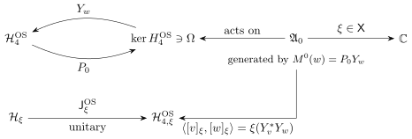
|
Figure 13. The spaces and maps of this
section. A positive word \(w\) in a slab gives the insertion
\(Y_w\) from the full ground space \(\ker H_4^{\text{OS}}\) of
the mixture, which need not be a line, into its OS space;
compression by the ground projection \(P_0\) gives \(M^0 (w)\),
and these operators generate the commutative algebra
\(\mathfrak{A}_0\). A phase is a character \(\xi\) of
\(\mathfrak{A}_0\). The OS space of the phase is the completion
of positive words under the form \(\xi (Y_v^{\ast} Y_w)\), the
value of \(\xi\) on the compression of a whole word, which need
not be the product of the values on its two halves |
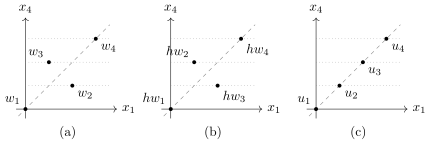
|
Figure 14. The axis exchange in the proof of Lemma 17.1, in the plane of the first and fourth coordinates, in units of \(j\); time \(x_4\) is vertical, and the dashed line is fixed by the exchange \(h\). (a) Four words, in time order \(w_1, w_2, w_3, w_4\). (b) After \(h\) the set of points is the same, but the transformed middle words have traded places, so the time order is \(hw_1, hw_3, hw_2, hw_4\). (c) On the diagonal, \(h\) moves no point and changes no time order; this identity removes \(h\) from the products. |
Rotations make spatial translations trivial at zero energy; compression then removes slab width and placement.
Lemma
Proof. For fixed words and large \(z^4\) the correlation is \(\langle v, U_{\vec{z}} e^{- (z^4 - c) H_4^{\text{OS}}} v' \rangle\), and strong heat convergence makes fixed time shifts negligible, uniformly in \(\vec{z}\). Choose an orthogonal reflection \(K\) taking \(y + e_4\) to \(|y + e_4 | e_4\). Since \(\langle K (y + e_4), Ke_4 \rangle = 1\), the ray \(tKe_4\) has positive time component. By the covariance of Lemma 16.17, rotating the displacements \(te_4 + y + e_4\) and \(te_4\) makes their difference purely temporal, so their correlations become equal in the limit; removing the extra \(e_4\) gives \(U_y P_0 = P_0\) by density.
The identities \(\textsf{B}_{h + t} (w) = \textsf{B}_h (w) e^{-
tH_4^{\text{OS}}}\) and \(\textsf{B}_{h + t} (\tau_{te_4} w) = e^{-
tH_4^{\text{OS}}} \textsf{B}_h (w)\) give width and placement
independence of \(M^0 (w)\), and \(M^0 (w) \Omega = P_0 [w]\), \(\langle
\Omega, M^0 (w) \Omega \rangle = S (w)\). Successive use of
| \(\displaystyle \lim_{j \to \infty} S (\tau_{z_1 (j)} w_1 \cdots \tau_{z_m (j)} w_m) = \langle \Omega, M^0 (w_1) \cdots M^0 (w_m) \Omega \rangle\) | (17.1) |
whenever \((z_{i + 1} (j) - z_i (j))^4 \to \infty\); in the induction, \(\psi_j \to \psi\) and \(t_j \to \infty\) imply \(U_{y_j} e^{- t_j H_4^{\text{OS}}} \psi_j \to P_0 \psi\) for arbitrary \(y_j\).
Commutativity. Let \(h \in O (4)\) exchange the first and fourth coordinates, and write \(hw\) for the word whose points, internal offsets included, and labels are transformed by \(h\), the labels through the representations of Lemma 16.17. Place four words \(w_1, \ldots, w_4\) at
with times \(0, j, 2 j, 3 j\) (Figure 14). The points
\(hz_i\) have times \(0, 2 j, j, 3 j\): the two middle words exchange
their time order. Covariance and
The right side still carries \(h\). Words \(u_k\) at the points \((k - 1) j (e_4 + e_1)\), \(k = 1, \ldots, 4\), which \(h\) fixes, keep their time order, so the same two identities give \(\langle \Omega, \prod_k M^0 (hu_k) \Omega \rangle = \langle \Omega, \prod_k M^0 (u_k) \Omega \rangle\). With \((u_k) = (w_1, w_3, w_2, w_4)\) this removes \(h\):
The vectors \(M^0 (w_4) \Omega = P_0 [w_4]\) span a dense subspace of
\(\ker H_4^{\text{OS}}\). By
Compression does not preserve products, and the identities used below
have separate jobs. For a positive word \(v\) in a slab of width \(h\)
put \(Y_v = \textsf{B}_h (v) |_{\ker H_4^{\text{OS}}}\), a bounded map
from \(\ker H_4^{\text{OS}}\) to \(\mathcal{H}_4^{\text{OS}}\). Then
\(M^0 (v) = P_0 Y_v\), and
| \(\displaystyle M^0 (\theta v \hspace{0.17em} w) - M^0 (v)^{\ast} M^0 (w) = Y_v^{\ast} (1 - P_0) Y_w \hspace{0.17em} .\) | (17.2) |
A character is multiplicative on \(\mathfrak{A}_0\), but a phase
evaluates a word at finite separation through the compression of the
whole word, \(S^{\xi} (\theta v \hspace{0.17em} w) = \xi (Y_v^{\ast}
Y_w)\). In the OS space of the phase, \(\xi (M^0 (v)^{\ast} M^0 (w)) =
\langle [v]_{\xi}, \Omega_{\xi}^{\text{OS}}
\rangle \langle
\Omega_{\xi}^{\text{OS}}, [w]_{\xi} \rangle\), so the character of the
right side of
Moment bounds in the vacuum state bound a compressed operator in every phase. This is the form in which lattice chessboard estimates enter here and in Sections 18–19.
Lemma
Proof. By Lemma 17.1, \(\langle \Omega, (U^{\ast} U)^n \Omega \rangle = \int | \xi (U) |^{2 n} \hspace{0.17em} d \nu (\xi)\). If \(| \xi_0 (U) | > b > B\), continuity gives an open neighbourhood \(O\) of \(\xi_0\) on which \(| \xi (U) | > b\), and full support gives \(\nu (O) > 0\). Then \(\nu (O) b^{2 n} \leqslant B^{2 n}\) for every \(n\), which is impossible. Gelfand theory identifies \(\|U\|\) with \(\sup_{\xi} | \xi (U) |\).\(\Box\)
The moment hypothesis comes from the lattice as follows. Let a lattice
word difference be interior with centered chessboard seminorm at most
\(B_0\) in one cell, multiplied by exterior insertions with centered
chessboard seminorms at most \(B_1, \ldots, B_L\) in disjoint finer
cells, and let \(U \in \mathfrak{A}_0\) be its compressed limit along
the ordered limit. Apply
A generic grid word has positions in \(a_k \mathbb{Z}^4\) with pairwise distinct coordinates along each axis. For real coefficient representatives \((d_i, c_i)\) write \(\langle \cdot \rangle_{N, p}\) for the Wilson expectation of Section 2.1, and put \(\mathcal{O}_{N, p} (w) = \prod_i O^{(d_i)}_{N, p} (c_i, x_i / a_N)\). The word differences used below are
| \(\displaystyle f_{j, N, p, T} =\mathcal{O}_{N, p} (\tau_{z_j (T)} w) -\mathcal{O}_{N, p} (\tau_{z_j (T)} \vartheta w), \qquad z_j (T) = Tja_k (1, 1, 1, 1) .\) | (17.3) |
For each degree bound and lower grid level \(m\), Lemma 14.30 chooses \(k \geqslant m\) before \(w\); these are the cofinal grids used below. For \(\varepsilon > 0\) it supplies real \(g_{j, N, p, T}\) and a finite \(R_{\varepsilon}\), independent of \(N, p, T, j\), with \(|g_{j, N, p, T} | \leqslant R_{\varepsilon}\) eventually in the ordered cutoffs for each fixed \(T, j\), and, for \(i < j\) and large \(T\), eventually in the ordered cutoffs, \(| \langle g_i g_j \rangle_{N, p} - \text{Re} \langle f_i f_j \rangle_{N, p} | \leqslant \varepsilon\); the threshold may depend on \(T, i, j\). Bounded \(g_i\) control the diagonal variance terms, for which \(f_i^2\) has no uniform bound.
Lemma
Each separated value is continuous in \(\xi\). For \(\nu\)-almost every \(\xi\), the time-axis OS ground space is one-dimensional.
Proof. Reflection and rotation invariance. We first prove
| \(\displaystyle M^0 (\vartheta w) = M^0 (w), \qquad M^0 (hw) = M^0 (w) \quad (h \in O (4)) \hspace{0.17em} .\) | (17.4) |
For a real grid word set \(Z = M^0 (w) - M^0 (\vartheta w)\). Equation
For fixed \(q, T\), intersect the finitely many eventual sets, take the
ordered cutoffs, then \(T \to \infty\). Each pair expands into four
separated moments, whose signed sum tends to \(a\) by Lemma 14.33,
Euclidean properties. Testing on positive words gives the permutation, unit and linearity identities and annihilates mixed null labels, so \(\mathcal{N}_d (S) \subset \mathcal{N}_d (S^{\xi})\). Character evaluation gives reality, covariance and smooth phase values, continuous in \(\xi\). For positive words \(w_i\) in a common slab write \(Y_i = Y_{w_i} : \ker H_4^{\text{OS}} \to \mathcal{H}_4^{\text{OS}}\). Since \(M^0 (\theta w_i w_j) = Y_i^{\ast} Y_j\),
The entries are compressions of whole words, not the products \(M^0
(w_i)^{\ast} M^0 (w_j)\) (see
Equal null spaces. Use the rows of Lemma 14.22, corrected lifts of Lemma 14.26 and coefficient limits of Lemma 15.5. Each row of trial \(\ell\) consists of a singleton \(u\) and optional spectator \(v\), placed at the comparison points \(r_{\ell} y^{\ell, i}\). Write \(\mathcal{G}_I^{\ell}\) for the Maxwell moment of the row labels in slots \(I\) at the unscaled points \(y^{\ell, i}\), and set \(s =\mathcal{G}^{\ell}_{\{u\}}\), \(s' =\mathcal{G}^{\ell}_{\{v\}}\) and \(c =\mathcal{G}^{\ell}_{\{u, v\}} - ss'\), omitting terms with \(v\) in singleton rows. In \(\mathfrak{A}_0\) put
The polynomials of
| \(\displaystyle \int_{\textsf{X}} | \xi (\Delta) |^{2 j} \hspace{0.17em} d \nu (\xi) \leqslant \gamma_{\ell}^{2 j} \qquad (j \in \mathbb{N}) \hspace{0.17em},\) | (17.5) |
and Lemma 17.2 gives \(| \xi (\Delta_1) |, | \xi (\Delta_1') |, | \xi (\Delta_2) | \leqslant \gamma_{\ell}\) in every phase. Expanding \(\Delta_2\) gives \(| \xi (M^0 (uv)) - ss' - c| \leqslant \gamma_{\ell} (1 + |s| + |s' |)\). The comparison has three parts of different kinds:
The inclusion is exact and was proved above, and with
Almost every ground space. Reflection positivity and E7 construct the phase heat semigroup as in Lemma 16.12. Write \([b]_{\xi}\) for a positive-word class and \(P_{0, \xi}^{\text{OS}}\) for its ground projection. Strong heat convergence and the mixture identity give, by dominated convergence,
the heat entries decreasing from their zero-time bounds. The integrands differ by \(\|P_{0, \xi}^{\text{OS}} [b]_{\xi} - S^{\xi} (b) \Omega_{\xi}^{\text{OS}} \|^2\), which therefore vanishes almost everywhere. Rational configurations and basis coefficients give a countable dense family in every phase OS space, by Gram continuity; outside the union of its null sets the ground range is \(\mathbb{C} \Omega_{\xi}^{\text{OS}}\).\(\Box\)
Choose \(\xi_{\ast}\) from the full-measure set of Lemma 17.3; only its ground-space dimension enters this choice, and it is retained throughout. The slab bound passes to every phase with the same constants, by transferring the repeated insertion estimate through the character and applying the power argument of Lemma 16.12.
Corollary
Proof. In the phase OS space put \(v_j = (A_{w^{\dagger}} A_w)^j v\). The mixed-space map \(Y (v_j) = \textsf{B} (v_j) |_{\ker H_4^{\text{OS}}}\) equals \((\textsf{B}_h (w)^{\ast} \textsf{B}_h (w))^j Y (v)\), so \(\|[v_j]_{\xi} \|^2 = \xi (Y (v_j)^{\ast} Y (v_j)) \leqslant \|Y (v)\|^2 \| \textsf{B}_h (w)\|^{4 j}\). The power argument gives \(\textsf{B}_h^{\xi} (w)\) of norm at most \(\| \textsf{B}_h (w)\|\), and the dense-vector argument gives its identities and norm derivatives.\(\Box\)
Proof of Theorem 6.13. Lemma 17.1 gives the character space, the full-support probability measure and the mixture formula. Lemma 17.3 gives E1–E7, equal null spaces, the common identities of Proposition 6.4 and Theorem 6.10, covariance and phase continuity.\(\Box\)
Use the response labels \(\mathcal{L}\) of Definition 2.12. With time reflection acting on labels through \(R_d\), the star is
| \(\displaystyle (\iota_d A)^{\ast} = \iota_d (R_d (\textsf{s}_4^{\text{refl}}) \bar{A}) \hspace{0.17em} .\) | (17.6) |
The boost generators \(- i \textsf{L}_d (K_{4 i})\) and the spatial
rotations integrate to \(SL (2, \mathbb{C})\), the simply connected
cover of \(SO^+ (1, 3)\); a full spatial turn acts trivially, so the
action descends to \(SO^+ (1, 3)\). Inclusions intertwine the actions,
and the time-reflection sign of \(K_{4 i}\) and antilinearity make the
star
Fix a phase \(\xi\). The reconstruction follows the scheme of
Osterwalder and Schrader [25, 26], with one
change: in place of their growth condition, the slab bounds of Lemma 16.12 and Corollary 17.4 give the strip bound
The requirements of Theorem 6.16 come from three sources. Reflection positivity gives the OS spaces, their heat semigroups and the positivity of the boundary distributions. Slab growth gives bounded insertions, hence the strip bound, tempered boundary values and continuity in the phase. The rotations of Lemma 16.17, continued to boosts, give Lorentz covariance and, through imaginary boosts, locality. Vacuum uniqueness first holds only for \(\nu\)-almost every phase (Lemma 17.3). The low-energy estimate of Lemma 17.9 is uniform in the phase; with the continuity in \(\xi\) of the vacuum-subtracted heat pairings and the full support of \(\nu\), it removes the exceptional set. That estimate, \(\mu_{A \Omega_{\xi}} \{0 < E \leqslant u\} \leqslant M_A u^2\), is polynomial in the energy: no positive lower bound on nonzero energies (spectral gap) is used or proved. Vacuum uniqueness is a statement inside one phase; nothing here shows that \(\nu\) is a point mass.
Positive-height operators give positive boundary distributions without a Euclidean extension across collisions.
Lemma
Here \(W^{\text{mix}}_n\) is the boundary distribution of the mixed continuation, defined below.
Proof. Positive imaginary times. Write \(e^{- tH_{4, \xi}^{\text{OS}}}\) for the phase heat semigroup. For a label \(a\) put \(B_{\xi, \epsilon} (a) = \textsf{B}_{2 \epsilon}^{\xi} (a (\epsilon e_4))\); Lemma 16.12 and Corollary 17.4 give \(\|B_{\xi, \epsilon} (a)\| \leqslant C_a \epsilon^{- q_a}\) for \(0 < \epsilon < 1\), uniformly in \(\xi\). For \(\text{Im} \hspace{0.17em} z > 2 \epsilon\) set \(G_{\xi, \epsilon} (z, y) = e^{- (\text{Im} \hspace{0.17em} z - 2 \epsilon) H_{4, \xi}^{\text{OS}}} e^{i \text{Re} \hspace{0.17em} zH_{4, \xi}^{\text{OS}}} U_y^{\xi}\), and for \(n \geqslant 1\)
with \(0 < \epsilon < 1\) and \(4 \epsilon < \min_j \text{Im} (z_{j + 1} - z_j)\); set \(\textsf{F}_0^{\xi} = 1\). At imaginary times the insertion rule gives \(S_n^{\xi}\), independently of \(\epsilon\), and the identity theorem extends this agreement. The function is holomorphic in the times and continuous in space; extend it by zero outside ordered times. Taking \(\epsilon = \delta / 8\) gives, uniformly in \(x\) and \(\xi\),
| \(\displaystyle | \textsf{F}_n^{\xi} (a ; x^4 + iy, \vec{x}) | \leqslant C \delta^{- m} \quad (0 < \delta \leqslant 1, y_{j + 1} - y_j \geqslant \delta) .\) | (17.8) |
Boundary distributions. Write \(\phi_{\xi} (y ; f) = \int
\textsf{F}_n^{\xi} (a ; x^4 + iy, \vec{x}) f (x)
\hspace{0.17em} dx\)
and \(\mathcal{G}= - i \sum_j j \hspace{0.17em} \partial_{x_j^4}\). By
The integrand is bounded by \(C \|\mathcal{G}^{m + 1} f\|_{L^1} / m\)!, uniformly in \(y, \xi\). At \(y = 0\) this defines \(W_n^{\xi}\), and dominated convergence gives every ordered boundary limit and a common Schwartz seminorm bound.
Dependence on the phase. The mixed operators of Lemma 16.12
define \(\textsf{F}^{\text{mix}}\) by
Lorentz covariance. Display the \(j\)th label in \(\phi_{\xi} (y ; f ; \ldots, a_j, \ldots)\). Differentiating Euclidean \((4, i)\) covariance and using the time Cauchy–Riemann identity gives
first at imaginary times, then by holomorphy. At the boundary
Spectral support. Define \(\tilde{W}_n^{\xi} (b) = W_n^{\xi} (\hat{b}_+ (- \cdot))\). For compactly supported smooth frequency tests \(b\), differentiating the height and the exponential multiplier gives cancellation, hence
| \(\displaystyle \tilde{W}_n^{\xi} (b) = \phi_{\xi} \left( y ; \widehat{(e^{\sum_j y_j p_j^4} b)}_+ (- \cdot)) \hspace{0.17em}, \right.\) | (17.10) |
including the zero endpoint. Sending ordered heights to infinity kills negative time-tail momenta, and translation and Lorentz covariance give support in \(\mathcal{V}_n\).
Positivity. Apply the propagators and insertions in
Locality is the exchange of two adjacent spacelike points. For \(1 \leqslant j < n\) let \(s\) be the transposition of \(j\) and \(j + 1\), write \(x^s\) and \(a^s\) for configurations and label lists with these entries exchanged, and put \(\mathcal{G}_j = \{x \in (\mathbb{R}^4)^n : \textsf{m} (x_{j + 1} - x_j) < 0\}\).
Lemma
The two orders give two holomorphic functions on two different tubes. Opposite imaginary boosts move a configuration with tied heights into the two tubes and so define two holomorphic germs at that configuration. At zero real times both germs restrict to the same Euclidean correlation, by permutation symmetry, so they coincide; the equality is carried to arbitrary real times, and partial boundary values give the claim.
Proof. The tube function. Let \(\mathcal{T}_n = \{w \in (\mathbb{C}^4)^n : \text{Im} (w_{k + 1} - w_k) \in V_+, k < n\}\), where \(V_+\) is the interior of \(\bar{V}_+\). Let \(\chi =\boldsymbol{1}_{\{ \text{dist} (p, \mathcal{V}_n) < 2\}} \ast \varrho_1\) with \(\varrho_1 \geqslant 0\) smooth, of unit integral and supported in the unit ball; then \(\chi = 1\) near \(\mathcal{V}_n\), has bounded derivatives, and vanishes at distance greater than three. For \(w \in \mathcal{T}_n\) define
With \(q_k = \sum_{l \geqslant k} p_l\), one has \(\sum_k p_k \cdot
\text{Im} \hspace{0.17em} w_k = \sum_{k \geqslant 2} q_k
\cdot \text{Im}
(w_k - w_{k - 1}) \geqslant c |p|\) on \(\mathcal{V}_n\), and up to a
bounded subtraction on \(\text{supp} \hspace{0.17em} \chi\); so the test
is a holomorphic family of Schwartz functions and \(\mathcal{W}_a\) is
holomorphic on \(\mathcal{T}_n\). By
Complex boosts. Real Lorentz covariance in Lemma 17.5 gives \(\mathcal{W}_a (\Lambda w) = \rho_n^{\vee} (\Lambda) \mathcal{W}_a (w)\) for real \(\Lambda\) and \(w \in \mathcal{T}_n\), where \(\rho_n^{\vee}\) acts on label tensors. For a spatial unit vector \(e\) and rapidity \(\beta\), the label action of the boost \(\Lambda_{\beta}\) along \(e\) is \(\exp (- i \beta \sum_i e_i \textsf{L} (K_{4 i}))\) on finite-dimensional spaces, an entire function of \(\beta\). Hence the covariance identity holds for complex \(\beta\), by the identity theorem in \(\beta\), whenever \(\Lambda_{\beta'} w \in \mathcal{T}_n\) along a path from \(0\) to \(\beta\).
Two germs. Fix heights with \(y_j = y_{j + 1}\) and \(y_k < y_{k + 1}\) for the other \(k\), and \(x \in \mathcal{G}_j\), so \(w_0 = x + iy\) lies on the boundary of \(\mathcal{T}_n\). Write \(x_{j + 1} - x_j = (\tau, \vec{v})\) with \(| \tau | < | \vec{v} |\) and put \(e = \vec{v} / | \vec{v} |\). The imaginary boost \(\Lambda_{ib}\) along \(e\) gives this difference the imaginary part \(\sin b \hspace{0.17em} (| \vec{v} |, \tau e)\), in time and space components, which lies in \(V_+\) for \(0 < b < \pi\); for small \(b\) the other differences stay in \(V_+\). So, for a small \(b_0 > 0\) and a small neighbourhood \(N\) of \(w_0\), \(\Lambda_{ib_0} w \in \mathcal{T}_n\) for \(w \in N\), and \(\Lambda_{ib} w \in \mathcal{T}_n\) for \(0 \leqslant b \leqslant b_0\) if moreover \(w \in \mathcal{T}_n\); the opposite boost \(\Lambda_{- ib}\) moves the exchanged configuration into \(\mathcal{T}_n\). Define, near \(w_0\),
Both are holomorphic in a neighbourhood of \(w_0\). By the complex boost identity along \([0, b_0]\), \(G_+ =\mathcal{W}_a\) on the part of that neighbourhood in \(\mathcal{T}_n\), and \(G_- (w) =\mathcal{W}_{a^s} (w^s)\) where \(w^s \in \mathcal{T}_n\).
The Wick slice. Suppose first that all real times of \(x\) vanish. Then \(w_0 = (iy_k, \vec{x}_k)_k\) is a separated Euclidean configuration, since \(\vec{x}_j \ne \vec{x}_{j + 1}\). The Wick slice \(\{(it_k, \vec{x}_k)\}\) is a real subspace of dimension \(4 n\) whose complex span is \((\mathbb{C}^4)^n\). Near \(w_0\) on the slice, points with \(t_j < t_{j + 1}\) lie in \(\mathcal{T}_n\), where \(G_+ = S^{\xi}_n (a ; \cdot)\); points with \(t_j > t_{j + 1}\) have exchanged configuration in \(\mathcal{T}_n\), where \(G_- = S^{\xi}_n (a^s ; (\cdot)^s) = S^{\xi}_n (a ; \cdot)\) by permutation symmetry. Since \(S^{\xi}_n\) is smooth at \(w_0\), all jets of \(G_+\) and \(G_-\) along the slice at \(w_0\), computed as limits from these open half-spaces, equal those of \(S^{\xi}_n (a ; \cdot)\). Real jets along the slice are restrictions of complex jets, and the slice spans \((\mathbb{C}^4)^n\); so all complex derivatives of \(G_+ - G_-\) vanish at \(w_0\), and \(G_+ = G_-\) near \(w_0\).
Propagation. For general \(x \in \mathcal{G}_j\) consider \(x (t) = (tx_k^4, \vec{x}_k)_k\), \(t \in [0, 1]\); it stays in \(\mathcal{G}_j\), since \(|t \tau | \leqslant | \tau | < | \vec{v} |\), and the strict height margins persist. Along this compact path both germs are defined at every point. Two germs of the same kind at nearby points agree on the overlap of their domains, since both extend the same function from the open set \(\mathcal{T}_n\) (respectively its exchanged image), which accumulates at each point. A finite chain of overlapping neighbourhoods carries \(G_+ = G_-\) from \(t = 0\) to \(t = 1\).
Partial boundary values. For \(f\) supported in a small ball around \(x \in \mathcal{G}_j\), the representation of \(W^{\xi}_{n, y}\) by the tube function and continuity up to the tied heights give \(W^{\xi}_{n, y} (a ; f) = \int G_+ (x' + iy) f (x') \hspace{0.17em} dx'\), and likewise \(W^{\xi}_{n, y^s} (a^s ; f^s) = \int G_- (x' + iy) f (x') \hspace{0.17em} dx'\). These agree, and a partition of unity gives \(W^{\xi}_{n, y} (a ; \psi) = W^{\xi}_{n, y^s} (a^s ; \psi^s)\) for compactly supported \(\psi\) with support in \(\mathcal{G}_j\); for general \(\psi \in \mathcal{S}_n\) with support in \(\mathcal{G}_j\), multiply by cutoffs equal to one on growing balls, which converge in \(\mathcal{S}_n\) without enlarging the support. Let the heights tend to zero along such tied height lists; continuity of the partial boundary distributions gives the claim.\(\Box\)
Lemma
Proof. Complete the form \(W^{\xi} (F^{\ast}
G)\) on \(\mathfrak{B}\) modulo null vectors to obtain
\(\mathcal{H}_{\xi}\), with \(\Phi_{\xi} (a, f) [b] = [(a, f) b]\). For
null \(x\) the inserted vector pairs with \(c\) as \(\langle x,
(a^{\ast}, \bar{f}) c \rangle = 0\); taking \(c\) to be that vector
preserves nullity and gives the adjoint law W1. Test continuity gives
strongly continuous covariance unitaries, and Lemma 17.5
gives W2. Translations integrate to a nondegenerate representation of
\(C^{\ast} (\mathbb{R}^4) = C_0 (\mathbb{R}^4)\) [19,
Theorem 3.7.11 and equation (3.89)] with spectral measure from [19,
Proposition 4.2.3], and the Fourier support in \(\mathcal{V}_n\) puts
the spectrum in \(\bar{V}_+\). Lemma 17.6, applied to
adjacent pairs inside vacuum expectations of words, gives W3 on the word
domain. The boundary condition of Definition 2.17 is the
definition of \(W^{\xi}_n\) in Lemma 17.5. A label acting
as zero has zero Euclidean correlations by
Surjectivity of the comparison map transfers ground-space information between the two Hilbert spaces.
Lemma
Proof. The map \(J : [b] \mapsto v_{\xi} (b)\)
of Lemma 17.5 is an isometry taking vacuum to vacuum and
intertwines spatial translations and heat by
The low-energy estimate is the infrared input of the reconstruction. For a fixed compactly supported local word \(A\), locality makes a commutator vanish outside a bounded spatial region for bounded times. An odd time average turns this into a positive spectral weight comparable to the energy \(E\) near zero. A momentum cutoff at scale \(u\) costs \(u^3\) in three spatial dimensions, and the cone \(| \vec{p} | \leqslant E\) gives \(u \hspace{0.17em} \mu \{u / 2 < E \leqslant u\} \lesssim u^3\); dyadic summation gives \(u^2\).
Lemma
where \(P_{0, \xi}\) projects onto \(\mathbb{C} \Omega_{\xi}\). Moreover \(\ker H_{\xi} =\mathbb{C} \Omega_{\xi}\) and \(\ker H_{4, \xi}^{\text{OS}} =\mathbb{C} \Omega_{\xi}^{\text{OS}}\).
Proof. The low-energy measure. Let
\(Q_{\xi} = \textsf{E}_{\xi} (\{\mathbf{p}^4 = 0\})\) be the full
zero-energy projection; until the last step its range is not assumed to
be a line. Let \(A^{\ast}\) be the word adjoint, reversing order and
applying the star
with \(\hat{\mu}_+ (z) = \int e^{ip \cdot z} \hspace{0.17em} d \mu (p)\). Write \(E = p^4\). The time average \(\bar{a} (y) = \int_0^1 [a (y, t) - a (y, - t)] / (2 i) \hspace{0.17em} dt\) is bounded by \(M\) and supported in \(\bar{B}_R\). It is the Fourier transform of two positive measures, the pushforwards of \(\varpi (E) \hspace{0.17em} d \mu\) under \(p \mapsto \vec{p}\) and of \(\varpi (E) \hspace{0.17em} d \mu^{\ast}\) under \(p \mapsto - \vec{p}\), where \(\varpi (E) = (1 - \cos E) / E\), \(\varpi (0) = 0\); on \(0 \leqslant E \leqslant 1\), \(\varpi (E) \geqslant E / \pi\). Choose a smooth momentum bump \(b_u\) with \(0 \leqslant b_u \leqslant 1\), equal to one on \(B_u\) and supported in \(B_{2 u}\); \(| \widehat{b_u}_+ (- y) | \leqslant 8 |B_1 | u^3\). Since \(| \vec{p} | \leqslant E\) on the spectral cone, \(b_u = 1\) on the shell \(\{u / 2 < E \leqslant u\}\), and Fourier inversion and positivity give
Summing the shells at \(u 2^{- j}\) gives
| \(\displaystyle \mu (\{0 < E \leqslant u\}) \leqslant CR^3 Mu^2 \qquad (0 < u \leqslant 1) \hspace{0.17em} .\) | (17.11) |
For \(u > 1\) use the total mass. Since \(e^{- sE} = \int_E^{\infty} se^{- st} \hspace{0.17em} dt\), Tonelli gives
From almost every phase to every phase. By Lemma 17.8,
\(\textsf{J}^{\text{OS}}_{\xi}\) is unitary and intertwines heat, so it
identifies \(\ker H_{\xi}\) with \(\ker H^{\text{OS}}_{\xi}\); by Lemma
17.3 both are \(\mathbb{C} \Omega_{\xi}\) for
\(\nu\)-almost every \(\xi\), and there \(Q_{\xi} = P_{0, \xi}\). The
vacuum-subtracted heat pairing \(\langle A \Omega_{\xi}, e^{- sH_{\xi}}
A \Omega_{\xi} \rangle - | \langle
\Omega_{\xi}, A \Omega_{\xi} \rangle
|^2\) is continuous in \(\xi\): by
Lemma
Proof. A scalar satisfies the relation by the adjoint law. Conversely, the adjoint law and iteration move words across matrix entries without requiring \(B\) to preserve the domain. For a word \(A\) put \(u = A \Omega_{\xi}\), \(v = A^{\ast} \Omega_{\xi}\) and, in the upper half-plane,
These are bounded and continuous to the boundary, where covariance and the weak relation give \(p (t) = q (- t)\). Morera and Liouville make their bounded pasted continuation constant, so \(\langle u, e^{- sH_{\xi}} B \Omega_{\xi} \rangle = \langle u, B \Omega_{\xi} \rangle\). Heat convergence and Lemma 17.9 give \(B \Omega_{\xi} = b \Omega_{\xi}\). Moving words again gives \(\langle A' \Omega_{\xi}, BA \Omega_{\xi} \rangle = b \langle A' \Omega_{\xi}, A \Omega_{\xi} \rangle\), so \(B = b 1\) by density.\(\Box\)
For the charge law set \(\eta = \text{diag} (- 1, - 1, - 1, 1)\), \(\zeta_i = 1\) for \(i \leqslant 3\), \(\zeta_4 = - i\), and
Let \(K (x) = k + Vx\) with \(V^{\textsf{T}} \eta + \eta V = 0\), and let \(\Sigma_K\) be its infinitesimal Lorentz label action. For real \(f \in C_c^{\infty} (\mathbb{R})\) of integral one and \(c \in C_c^{\infty} (\mathbb{R}^3)\) put \(Q_K (f, c) = \sum_b T^{\text{M}}_{4 b} (K^b (c \otimes f))\). Suppose \(g \in C_c^{\infty} (\mathbb{R}^4)\), and \(c = 1\) on a ball such that all \((y, s)\) over its complement, \(s \in \text{supp} \hspace{0.17em} f\), are spacelike to \(\text{supp} \hspace{0.17em} g\). The charge law is
| \(\displaystyle i [Q_K (f, c), \Phi_{\xi} (\iota_d A, g)] = \Phi_{\xi} (\Sigma_K \iota_d A, g) - \sum_a \Phi_{\xi} (\iota_d A, \partial_a (K^a g)) \hspace{0.17em} .\) | (17.13) |
A common polynomial bound permits the continuation of local stress identities.
Lemma
Proof. Tensor properties. The factors
give \(T^{\text{M}}_{44} = T_{44}\), \(T^{\text{M}}_{4 i} = iT_{4 i}\),
\(T^{\text{M}}_{ij} = - T_{ij}\). Euclidean symmetry and
The Euclidean jump. For real \(c\), insert \(c (y) h (t - t_0)\) into the shell identities of Theorem 6.10, transferred to the phase by Lemma 17.3, and integrate conservation on each side of \(t_0\). The \(\nabla c\) term stays away from the distinguished point and remains bounded, so \(\sum_b \int c (y) K_{\text{E}}^b (y, t) T_{4 b} (y, t) \hspace{0.17em} dy\) is Cauchy on each side, with jump \(\Sigma_K A + \sum_b K_{\text{E}}^b \partial_b A\), where \(K_{\text{E}}^b (y) = \zeta_b K^b (\vec{y}, iy^4)\).
Continuation of the jump. Fix strictly ordered heights \(y_j\) for all fields other than the current, including the distinguished field with index \(0\). For their real times \(t_j\) put \(z_j (\varsigma) = iy_j + \varsigma t_j\), and place the current at \(z_0 (\varsigma) \pm i \varepsilon\), retaining Euclidean separation \(\varepsilon > 0\). Write
where \(\textsf{F}_{\pm}\) inserts the current immediately after or
before the distinguished field. Choose a complex neighbourhood
\(\mathcal{U}\) of \([0, 1]\) preserving the other strict height
differences. On \(\text{supp} \hspace{0.17em} \nabla c\) the spacelike
germs of Lemma 17.6 bound the side integrals, uniformly for
small \(\varepsilon\) and \(\varsigma\) in compact \(L \subset
\mathcal{U}\), and conservation gives \(\sup_{\varsigma \in L}
|I_{\varepsilon}^{\pm} (\varsigma) -
I_{\varepsilon'}^{\pm} (\varsigma)
| \leqslant C_L | \varepsilon -
\varepsilon' |\). The limits are
holomorphic; at small imaginary \(\varsigma\) the Euclidean calculation
identifies their jump, and the identity theorem extends it to
\(\varsigma = 1\). Test against \(g, f\) and take the continuous partial
boundaries; integration by parts differentiates \(K^a g\), giving
Proof of Theorem 6.16. Lemmas 17.5, 17.6 and 17.7 give, in every phase, a faithful theory satisfying W1–W3 and the spectral condition, with continuations satisfying Definitions 2.16 and 2.17. Lemma 17.8 gives the unitary comparison, Lemma 17.9 the vacuum lines and hence W0, and Lemma 17.10 the scalar weak commutant. Lemmas 17.9–17.11 also give the uniform rates and the continued stress, at the retained phase \(\xi_{\ast}\) as at every other.\(\Box\)
This section proves Theorem 6.18 and the non-free comparisons. The stress tensor \(T\) of Section 16 is normalized by its comparison with the free Maxwell stress (Proposition 6.11), and the free stress is traceless. So this comparison cannot determine the first nonzero trace term, which is smaller by the inverse running coupling (Table 9). That term corresponds to the one-loop trace anomaly [9]; we compute its coefficient from a lattice Ward identity, with a rate. The proof of Theorem 6.18 has five steps.
\(L = T^{\text{Max}}\), \(D = \delta_{ab} \mathcal{O}_{F^2}\) and
\(\Xi\) span the centered real symmetric \(H_4\)-tensorial tensors
of degree four; a functional \(\rho_{\text{tr}}\) reads the trace
from the divergence
A lattice stress current (Definition 18.4) has
divergence equal to the action variation up to a defect, which block
transfer
Lemma 18.5 computes the regulated Ward coefficient \(- 12 \kappa_G\). Lemma 18.7 carries it to continuum fields along the radii of Lemma 18.3, with the rate of Lemma 18.6.
A conserved combination of these fields is a multiple of \(T\); its \(D\)-coefficient tends to \(d_2 = - \kappa_G / 4\) (Proposition 18.8).
Positivity makes \(G_{\Theta}\) nonincreasing. This turns comparison along subsequences, which uses frames, into the frame-free limit at every radius (Figure 15).
Section 18.2 proves the non-free comparisons, each with its comparison class: no two-point statement excludes a generalized free field with the same spectral measure. In the selected phase, on no interval \((0, \delta)\) does \(G_{\Theta}\) agree with a finite Wick profile (Proposition 6.19).
Throughout, retain the fields, inclusions and units of Definition 2.12 and Proposition 6.4, the tensor of Theorem 6.10, and the selected reconstruction of Theorem 6.16. The symbols \(\tau, e_{\text{tr}}, \Theta, G_{\Theta}\) and \(A_G\) have the meanings of Definition 6.17. Write \(\Phi_{\Theta} (f) = \Phi (\iota_4 \Theta, f)\), and use the word domain of item W1 of Definition 2.14.
Centering must hold on the common operator domain, as well as in separated correlations. The proof below identifies the subtraction after continuation.
Lemma
Proof. Unit deletion (Definition 2.9) and the quotient calculus of Lemma 15.5 remove the unit insertion; the continuation of Lemma 17.5 and the field realization of Lemma 17.7 carry this to the operators. Deleting the unit insertion leaves a Euclidean correlation independent of its position. On each ordered-time region its continuation is therefore constant in that variable. The identity theorem on the connected continuation domain \(\mathcal{Z}_n\) of Definition 2.16, applied successively in each time variable, identifies it with the correlation containing the unit. Boundary values and smearing give \(\langle u, \Phi (\iota_4 \boldsymbol{1}_4, f) v \rangle = (\int f) \langle u, v \rangle\) for word vectors \(u, v\). Density and linearity give the identity. The zero Euclidean one-point function continues to zero and has zero boundary distribution, proving the centering assertion.\(\Box\)
We use the Fourier convention of Section 6.4:
In particular, \(\mathcal{W}_{\text{rel}} (\bar{f} \otimes h) = \overline{\hat{f}_+} \hat{h}_+\). Write \(W_2^{\xi_{\ast}} (\Theta, \Theta ; \bar{f} \otimes h) = \langle \Phi_{\Theta} (f) \Omega, \Phi_{\Theta} (h) \Omega \rangle\) for the joint tempered boundary distribution of Lemma 17.5. The next lemma constructs its positive measure.
Lemma
It is Lorentz invariant in momentum variables, and
Proof. The measure is built from the positive boundary distributions of Lemma 17.5. For \(v_f = \Phi_{\Theta} (f) \Omega\), translation covariance gives \(\hat{h}_+ (P) v_f = \hat{f}_+ (P) v_h\). Here \(\hat{h}_+ (P) = \int \hat{h}_+ (\mathbf{p}) \hspace{0.17em} d \textsf{E} (\mathbf{p})\), with \(\textsf{E}\) the joint translation spectral resolution of Theorem 6.16. Both sides smear the field with \(f \ast h\). Choose tests whose transforms do not vanish on successively larger balls. On such a ball define \(d \mu_{\Theta} = | \hat{f}_+ |^{- 2} d \mu_{v_f}\). The displayed identity makes these definitions agree on overlaps. Polarization gives \(\langle v_f, v_h \rangle = \int \overline{\hat{f}_+} \hat{h}_+ \hspace{0.17em} d \mu_{\Theta}\). Product tests determine the joint distribution.
The spectrum condition gives cone support. Schwartz continuity, applied to inverse transforms of cutoffs equal to one on \(\{|\mathbf{p}| \leqslant R\}\), gives \(\mu_{\Theta} (\{|\mathbf{p}| \leqslant R\}) \leqslant C (1 + R)^k\). Lemma 17.11 continues \(T\) to a symmetric Hermitian Lorentz tensor. Contraction and invariance of the unit (Lemma 16.17) make \(\iota_4 \Theta\) a Hermitian Lorentz scalar. Covariance of \(W_2\) and uniqueness of the measure give Lorentz invariance.
Tempered growth and \(|\mathbf{p}| \leqslant \sqrt{2} \mathbf{p}^4\) on
the cone make the Fourier–Laplace integral holomorphic at positive
imaginary time, with boundary \(W_2\). To identify it with the Euclidean
continuation of Lemma 17.5, take enough primitives to
obtain continuous boundary values, using the polynomial boundary bound
The next lemma extends Lemma 16.8 to prescribed radii. Its
proof also transfers the derivative argument of
Lemma
the couplings satisfy
| \(\displaystyle \beta_i \to \infty, \qquad \frac{\log (1 / r_i)}{\beta_i} \to \kappa_G^{- 1} \hspace{0.17em} ;\) | (18.1) |
for every arity \(n_{\text{ar}} \geqslant 1\), degrees \(d_j \leqslant D\), labels \(A_j^{(i)} \to A_j\) and compact \(\mathcal{K} \subset \text{Gen}_{n_{\text{ar}}}\),
and the same holds for each fixed jet and translation-shell flux;
for \(n_{\text{ar}} = 2\) without derivatives, (ii) holds uniformly over the phases.
Proof. The proof follows the finite-dimensional construction of Lemma 16.8, with radii placed in comparison windows. The source estimates of Lemmas 14.24 and 14.14 control the windows, and Lemma 14.27 moves the insertion points.
Radii and levels. Put \(M_n = M^{\text{cut}}_n\). At radius level \(n\) allow
| \(\displaystyle r (n, u) = a_n M_n^u, \qquad u \in [\alpha_0, \alpha_0 + 1], \qquad k (n) = \min \{m > n : \log (a_n / a_m) \geqslant (\log \hat{\beta}_n)^{48} \} \hspace{0.17em} .\) | (18.2) |
The separation in \(k (n)\) leaves room for all fixed-degree marked transports; its logarithmic size is negligible compared with \(\hat{\beta}_n\). For degree \(D\) and an arity bound \(n_{\text{ar}} \geqslant 2\) choose comparison exponents \(\alpha_0, \alpha_1, \alpha_2\) and \(c\) with
Choose the differences \(\alpha_0 - \alpha_1 > 6\), then \(- c > (\alpha_0 - \alpha_1) Dn_{\text{ar}}\), then \(\alpha_0 - \alpha_2 > 5 - c\), and finally increase all three \(\alpha_j\) together until \(\alpha_2 \geqslant Dn_{\text{ar}} + 10\).
Comparison windows. We first obtain comparison windows at every sufficiently late radius level, rather than only the intervals selected in Lemma 14.2. For each of the three exponents \(b = \alpha_j + u - \alpha_0\), stop backwards from \(n\) when the accumulated logarithmic block length first exceeds \((b + 2) \log M_n\), then stop again after another \(10 \log B_n\). The entry bounds fixed in Section 14.1 give \(\ell_m \leqslant \log \hat{\beta}_m\) at every level \(m\). Each overshoot is therefore \(O (\log \log \hat{\beta}_n) = o (\log M_n)\), so the resulting cell side is at most \(a_n M_n^{b + 5}\). All levels in these windows tend to infinity and their couplings have ratio tending to one. The accumulated source loss satisfies
by
Chessboard seminorms. At its own normalization a singleton
therefore has chessboard seminorm at most \(1 + |S^{\text{Max}}_1 (A)
|\). Indeed coefficient extraction at amplitude \(e^{2 q}\), \(q = \log
M_n / (16 n_{\text{ar}})\), bounds its centered seminorm by \(e^{q - 2
q} \leqslant 1\). Expand a degree-\(D\) label in weight-homogeneous
basis vectors. Changing from exponent \(\alpha_1 + u - \alpha_0\) to
\(u\) multiplies a weight-\(j\) coordinate by \(M_n^{(\alpha_0 -
\alpha_1) j}\), hence bounds this seminorm by \(CM_n^{(\alpha_0 -
\alpha_1) D}\). Include all signed and conjugated basis vectors in the
finite comparison request. The chessboard inequality
These are the contributions of coordinate-coincidence strips of width
\(4 \delta_n\) and interpolation across one mesh cell; include a strip
for each coordinate hybrid, a finite union of volume \(O (\delta_n)\)
since \(h^{\text{mesh}}_n = o (\delta_n)\). Both vanish uniformly in \(u
\in [\alpha_0, \alpha_0 + 1]\) by the choice of the comparison
exponents. For the remaining error, use the corrected Gaussian source of
Lemma 14.24 on every subset of the \(n_{\text{ar}}\) slots,
as in
Phase uniformity. By Lemma 17.2 and the lattice paragraph after it, these seminorm bounds on every repeated reflected product bound the norm of the corresponding compressed zero-energy operator, hence its value at every character of the phase algebra of Theorem 6.13. This gives (iii), including moving coefficients by finite-dimensional multilinearity.
Every small radius lies in a window. By the same entry bound
\(\ell_m \leqslant \log \hat{\beta}_m\), applied to both adjacent stage
ratios, \(\ell_n \leqslant M_{n + 1}\) eventually. Monotonicity of
\(M_n\) gives \(r (n, \alpha_0) \leqslant r (n + 1, \alpha_0 + 1)\),
while \(r (n, \alpha_0) \to 0\). First crossing of any prescribed small
radius, followed by continuity in \(u\), puts that radius in one of
these intervals. Diagonal extraction over degrees, arities, compact sets
and jet orders gives \(n_i, k_i = k (n_i)\) and frames, using Lemma 14.8 for symmetries and units and the recursive correction
Jets and couplings. For jets, the argument of
By that proof, these three tensors span the centered real symmetric \(H_4\)-tensorial tensors of degree four.
Write \(\langle F_{ac}, F_{bc} \rangle = \sum_{\alpha} : F^{\alpha}_{ac} F^{\alpha}_{bc}\): and similarly with derivatives. Before imposing the Maxwell equation, divergence has three coordinates, represented in component \(b\) by
For diagonal entries \(z_0 \sum_c \langle F_{ac}, F_{ac} \rangle + z_1 \sum_{b, c} \langle F_{bc}, F_{bc} \rangle\) and off-diagonal entries \(z_2 \sum_c \langle F_{ac}, F_{bc} \rangle\), the divergence coordinates are \((2 (z_0 - z_2), 2 z_1 + z_2 / 2, z_2)\). Indeed Bianchi gives \(\sum_{a, c} \langle F_{ac}, \partial_a F_{bc} \rangle = \frac{1}{2} \sum_{a, c} \langle F_{ac}, \partial_b F_{ac} \rangle\). Thus the functional \(\rho_{\text{tr}} (x, y, z) = - 2 x - 8 y\) satisfies
It annihilates the third coordinate, the Maxwell equation direction. Write \(R_5 \cong \mathbb{R}^3\) for this raw space and \(V_5\) for the space of real \(H_4\)-covariant axis vectors in \((M_5^{\text{Max}})^4\). The free Maxwell quotient map \(s : R_5 \to V_5\) is onto, with \(\ker s =\mathbb{R}v_{\text{eom}}\), \(v_{\text{eom}} = (0, 0, 1)\) and \(\rho_{\text{tr}} (v_{\text{eom}}) = 0\); thus \(V_5\) is two dimensional.
Definition
With \(\nabla_a = \sum_{j = 1}^4 c^{\nabla}_j (\textsf{s}_a^j - \textsf{s}_a^{- j})\) and \((c^{\nabla}_1, c^{\nabla}_2, c^{\nabla}_3, c^{\nabla}_4) = (4 / 5, - 1 / 5, 4 / 105, - 1 / 280)\), the Ward defect is \(\mathcal{E}_b = \sum_a \nabla_a J_{ab} - D \textsf{S} [Y_b]\).
The current \(J\) is the lattice form of \(T^{\text{Max}}\), and \(Y_b\) is the initial left displacement. Initially \(\text{tr} \hspace{0.17em} J = 0\) and \(J_{ab} - J_{ba} = 0\), so these data satisfy the identities (a)–(b) of Lemma 18.5 below with \(q = 0\) and \(\textsf{t} = 0\).
Here \(\textsf{G}_a^{(\ell)}\) is \(\textsf{G}_a\) with every shift replaced by its \(\ell\)th power, and \(\textsf{G}_a \hspace{0.17em} (\textsf{s}_a - 1) = \nabla_a\). Put \(\textsf{K}_a = \textsf{G}_a \textsf{M}_a \prod_{c \ne a} \textsf{M}_c \textsf{N}_c\) and \(\textsf{K}_a^{\text{edge}} = \textsf{N}_a \prod_{c \ne a} \textsf{M}_c \textsf{N}_c\). Since \(\textsf{M}_a (\textsf{s}_a - 1) = \ell^{- 1} (\textsf{s}_a^{\ell} - 1)\),
The last quotient is a finite Laurent polynomial: \(\textsf{G}_a - \textsf{G}_a^{(\ell)} \textsf{M}_a\) vanishes modulo \(\textsf{s}_a^{\ell} - 1\) after multiplication by \(\textsf{M}_a\), because \(\textsf{M}_a\) averages all residue classes and both factors \(\textsf{G}_a, \textsf{G}_a^{(\ell)}\) have mass one. Polynomial division defines \(\textsf{K}_a^{\text{tr}}\). The support radius of \(\textsf{K}_0\) is at most \(56 \ell\), its mass is one and its absolute coefficient sum is at most \(32^4\).
For Lemma 11.6's stationary background \(U_{\text{stat}} (V)\), stationary substitution is \(\mathcal{I}F (V) = F (U_{\text{stat}} (V))\). The stationary equation is \(D_U (\textsf{S} + \textsf{S}_{\text{block}}) = 0\) on the gauge-fixed fine variations. Retain the stationary coarse frame \(h_{\text{fr}}\) from the coordinates preceding Lemma 11.7, and write \(Q^{\text{pred}} (U) = (Q_e^{\text{pred}} (U))_e\) and \(\tilde{Q} (U, h) = (Q^{\text{pred}} (U))^h\) for the predictor in that frame. Its fine-coordinate differential is
For the root correction, let \(\varrho_x (y ; \eta)\) be minus the uniform average of the signed sums of \(\eta\) over the frame routes from \(y\) to the patch points, as in the proof of Lemma 11.6. Define scalar coefficients \(b_{x, e}\) by
Let \(g_{x, e} = h_{\text{fr}} (x) U (\gamma_{x, e})\), where \(\gamma_{x, e}\) is the fixed coordinate route from the embedded root \(x\) to \(e^-\). The root map and its coarse gauge variation are
These formulas transport a fine displacement to the predictor and correct its root frame. Evaluate them at the stationary pair and set \(\mathcal{I}_{\ast} Y = (R_f + d_V R_0) Y (U_{\text{stat}} (V))\). With \(\delta_a = \textsf{s}_a - 1\), transfer by
Starting with \(q_a = 0\), this preserves \(\text{tr} \hspace{0.17em} J = \sum_a \delta_a q_a\). The antisymmetric part, which need not remain zero, is likewise a sum of forward differences: its new correction in direction \(a\) is \(\ell^4 \textsf{K}_a^{\text{tr}} \mathcal{I}J_{ab}\) and in direction \(b\) is \(- \ell^4 \textsf{K}_b^{\text{tr}} \mathcal{I}J_{ba}\), in addition to the transferred old differences.
For an analytic local function \(F\), its degree-\(d\) Taylor map \(\text{Tay}_d \hspace{0.17em} F\) (Section 2.3) is, on a radial jet \(\textsf{j}\), \(\sum_{v = 0}^d [\varepsilon^v] F (U (\text{sc}_{\varepsilon} \textsf{j}))\), in the basis of Definition 2.7. The weighted Taylor map is \(t_m^{\textsf{N}} \text{Tay}_d \hspace{0.17em} F\), with the factor-count operator of Definition 2.8. Symmetrize \(J\), average over \(H_4\) and conjugation, apply the degree-four Taylor map and marked transport, and subtract the mixture mean. Call the resulting field \(B_i^L\). The same operations on the local contractions defining \(\Xi, D\) give \(B_i^{\Xi}, B_i^D\).
Fix a colour \(\alpha\). For a family \(F_b\) write
Coefficients use \([z^r t^s] F = (r!s!)^{- 1} \partial_z^r \partial_t^s F (0)\). Put \(\textsf{h} (F) = \textsf{l} (F) - \frac{1}{2} \text{Re} \sum_{a \ne c} [z^2] \widehat{F_c}_{c \alpha, c \alpha} (ze_a, - ze_a)\). The Haar coefficient is \(\mathfrak{h} (Y) = \textsf{h} (\text{div}_{\text{Haar}} \hspace{0.17em} Y)\); the subtraction corrects the lattice derivative. Define
where \(H\) is the left Hessian of \(\textsf{S}\) and \(d\) is the infinitesimal gauge insertion. For \(a > 0\) and \(r \in \mathbb{N}\), with \(\|x\| = |x|_{\infty}\) in the kernel's lattice units, put
For a chart function anchored at \(o\), its weighted order-\(r\) seminorm is the sum of absolute link coefficients of \(D^r F (0)\) against \(\prod_{v = 1}^r \vartheta_{a, r} (e_v^- - o)\); for a displacement use its link components. These weights control the spatial moments in the momentum derivatives below. Write \(F \equiv_4 G\) if the field derivatives of \(F\) and \(G\) at zero agree through order four. The next lemma computes the scalar coefficient; its proof follows.
Lemma
\(D \textsf{S} [Y_b] \equiv_4 \sum_a \nabla_a J_{ab} -\mathcal{E}_b\);
\(\text{tr} \hspace{0.17em} J = \sum_a \delta_a q_a\) and \(J_{ab} - J_{ba} = \sum_c \delta_c \textsf{t}_{abc}\);
the \(a\)-weighted seminorms of orders \(2\)–\(4\) of \(J, Y, q, \textsf{t}\) are at most \(C\);
those of \(\mathcal{E}\), and the deviations of the zero-field Hessians of \(J\) and \(Y\) from their free values on tests of weight at most \(4\) and \(5\), are at most \(\varepsilon_{\nu} \to 0\).
Then, for every colour, \(\mathfrak{h} (Y^{(\nu)}) \to - 12 \kappa_G\).
Proof. The inputs are the normalization of \(\kappa_G\) (Definition 2.1), the kinetic and quadratic cancellations and the classical matching of the path action (Lemmas 12.4 and 12.6), and the one-loop coefficient of Lemma 12.9. Write \(\mathcal{R}_{\mu} = (H + dd^{\ast} + \mu^2 I)^{- 1}\), \(\mathcal{G}_{\mu} = (d^{\ast} d + \mu^2 I)^{- 1}\). For \(\Psi_s (U) = e^{sY (U)} U\) let \(\mathcal{Y}_U (z) = \partial_s |_0 \log (\Psi_s (e^z U) \Psi_s (U)^{- 1})\) and \(\mathcal{V}= D\mathcal{Y}_U (0)\). If \(\mathcal{J}_U\) is the mixed derivative of \(\log (\text{gauge}_{e^v} (e^z U) U^{- 1})\) in \(v, z\) at zero, gauge invariance gives \(Hd = -\mathcal{N}\), \(\mathcal{N}= D \textsf{S} [\mathcal{J}_U]\), hence
The product rule for \(D^2 (D \textsf{S} [Y])\) and cyclicity of trace now give
with \(Z = \frac{1}{2} \text{contr} (\mathcal{R}_{\mu}, D^2 \mathcal{Y}_U (0)) - \text{contr} (\mathcal{G}_{\mu} d^{\ast} (\mathcal{V}+\mathcal{V}^{\ast})\mathcal{R}_{\mu}, \mathcal{J}_U)\). Contractions sum the indicated matrix indices.
Cancellation. The leading quadratic kernel of an invariant scalar action at the required momentum order is a colour multiple of \(|p|^2 I - p \otimes p\). Write \(X_{acb}\) for the coefficient of momentum \(e_a\) in the diagonal polarization-\(c\) entry of \(DY_b\), with its colour indices contracted against the action kernel. Gauge covariance makes the mixed polarization term \(- X_{cac}\) and gives \(X_{aaa} = 0\). In the tested variation the three terms, after summing the intermediate polarization, are
Summing over \(a \ne c\) makes the first and second sums \(- 3 \sum_{b,
c} X_{bcb}\), cancelling the third sum. Higher momentum orders do not
contribute. This applies to \(D \Gamma_{\mu} [Y]\), \(D \textsf{S} [Z]\)
and the further action variation below, uniformly on each fixed \(\mu
\in [\delta, 1]\). For the first term on the left of
The regulator term. For \(\chi (x) =\boldsymbol{1}_{x = 0}\) define \(M_b h (x) = \chi (x) h_b (x)\), \((D_b h)_a (x) = \delta_a \chi (x) h_b (x)\) and \((T_b^{(r)} h) (x) = \delta_b \chi (x) h (x)\) on \(r\)-forms, \(r = 0, 1\). Set
where \(\text{sym} \hspace{0.17em} A = (A + A^{\ast}) / 2\). The inverse identity above yields
The tested \(D_b\) term tends to \(\textsf{q} (\text{tr} \hspace{0.17em} \mathcal{R}_{\mu})\); each of the four \(T_b^{(r)}\) terms tends to \(\textsf{q} (\text{tr} \hspace{0.17em} \mathcal{R}_{\mu})\) or \(\textsf{q} (\text{tr} \hspace{0.17em} \mathcal{G}_{\mu})\) respectively. This follows by summing \(\delta_b \chi\) against the two Fourier waves: its symbol is \(e^{- it} - 1 = - it + O (t^2)\), paired with the factor \(i\) in \(\textsf{l}\). Translation invariance identifies the local anchor sum with the volume-normalized trace in \(\textsf{q}\). Consequently their sum is \(- \textsf{q} (\text{tr} \hspace{0.17em} \mathcal{R}_{\mu}) + 2 \textsf{q} (\text{tr} \hspace{0.17em} \mathcal{G}_{\mu})\). Differentiation of \(\Gamma_{\mu}\) in \(\mu\) gives the same expression multiplied by \(\mu^2\), namely \(\mathcal{D}_{\Lambda} (\mu)\). We have proved
| \(\displaystyle \mathfrak{h} (Y) =\mathcal{D}_{\Lambda} (\mu) + \mu^2 \textsf{l} (\text{Rem}) + o (1),\) | (18.6) |
with error uniform on every fixed \([\delta, 1]\).
For the remainder, the inverse-kernel argument in the proof of
The proof of
Lemma
Proof. Put \(k_i = v_i - t_i s_i v_i\). Then \(s_i k_i = 0\), and \(k_i \to v\) since \(t_i\) is bounded and \(s_i v_i \to 0\). The maps \(\Phi_i (h, c) = t_i h + ck_i\) from \(H \times \mathbb{R}\) to \(E\) converge to \(\Phi (h, c) = th + cv\), which is injective (apply \(s\)) and hence invertible, as \(\dim E = \dim H + 1\). So \(\Phi_i^{- 1} \to \Phi^{- 1}\); since \(s_i \Phi_i (h, c) = h\), also \(s_i \to s\). For \(y \in E\) write \(\Phi_i^{- 1} y = (s_i y, c_i (y))\), so that \(y - t_i s_i y = c_i (y) k_i\) and \(|c_i (y) | \leqslant C \|y\|\) uniformly in \(i\). Then
Hence \(e_i \| \lambda_i s_i - \rho \| \leqslant C \left( e_i | \rho (v_i) | +\| \rho \| \sup_j \|t_j \| \hspace{0.17em} e_i \|s_i v_i \| \right) \to 0\). Boundedness of \(\lambda_i\) follows from \(t_i \to t\).\(\Box\)
|
|||||||||||||||
Lemma
and the tensors satisfy
Thus \(\lambda_i\) reads \(\rho_{\text{tr}}\), that is \(- 4\) times the \(D\)-coefficient, of a divergence with error \(o (E_i^{- 1})\), and its value on the stress divergence, of size \(O (R_i)\), is the coefficient of Lemma 18.5 divided by \(12\).
Proof. We verify the hypotheses of Lemma 18.5 for the transferred current, compute the finite coefficient at each level, and read it along the radii of Lemma 18.3. The stationary kernels (Lemmas 11.6–11.10) control the transfer, and Lemmas 14.7–14.9 control marked transport.
The proof has five parts, and each has its own reason for smallness (Table 10). The current estimates are a contraction under repeated block transfer. The finite coefficient is accurate because of the thresholds and the exponential tails. The trace of the current is an exact forward difference; this, with the matching gain of marked transport, gives the equation direction its rates, and Lemma 18.6 turns that rate into the accuracy of \(\lambda_i\). The tensor traces are small for a different reason: the same forward difference becomes small after averaging over many sites. No single power count covers all five. The choices are made in this order: the block ratios and entry couplings of the stages, once and for all, so that transfer contracts; at a fixed level \(k\), the transfer depth and the period; then the ordered limit at that \(k\); and finally \(k = k_i\) along the radii. Since \(M^{\text{cut}}_k = e^{h_k}\) with \(h_k = (\log \log \hat{\beta}_k)^2\), the multipliers of the statement are \(E_i = (M^{\text{cut}}_{k_i})^{1 / 5}\) and \(R_i = (M^{\text{cut}}_{k_i})^{1 / 6}\).
|
||||||||||||||||||||||||
Table 10. The five parts of the proof of Lemma 18.7. The readout error \(o (E_i^{- 1})\) is multiplied by coefficients of size \(O (R_i)\), and \(R_i / E_i \to 0\). |
Current estimates. The transfer identities give (a)–(b) of Lemma 18.5; we prove (c)–(d) below. Differentiating the stationary equation eliminates its fine variation. Fourth-order matching in Lemma 12.6 preserves \(\sum_a \nabla_a J_{ab} -\mathcal{E}_b \equiv_4 D \textsf{S} [Y_b]\). The kernel identities above preserve the trace and antisymmetric parts as differences. Work after stage \(j \geqslant 7\) and choose \(0 < a < c_j\), with \(c_j\) the kernel decay exponent of Lemma 11.6. Its kernel bound applies through polynomial degree three. Divide the order-\(r\) current defect by \((\log \hat{\beta}_m)^r\). At orders \(r = 3, 4\), the linearized stationary fields contribute \(\ell^{- 2}\) each, so transfer costs \(C_j \ell^{5 - 2 r}\). At order two the matched low-momentum terms must first be removed. The affine and quadratic parts of a stationary test field have weighted sizes \(C_j (1 + |x|) / \ell^2\) and \(C_j (1 + |x|)^2 / \ell^3\); the remainder is at most \(C_j (1 + |x|)^3 / \ell^4\), by Lemmas 11.6 and 11.9. Without the subtraction, the affine–affine and affine–quadratic products, with factors \(\ell^{- 4}\) and \(\ell^{- 5}\), would cost \(\ell\) and \(1\) after multiplication by \(\ell^5\), and transfer would not contract them. Subtracting them leaves quadratic–quadratic and affine–remainder products, each with factor \(\ell^{- 6}\). Multiplication by \(\ell^5\) gives \(C_j / \ell\). A bounded matched contribution gives the additional \(C_j / (\log \hat{\beta}_m)^2\). More precisely the order-two factor is bounded by
Both terms are small once the ratio and the coupling are large. Thus the three orders gain for different reasons: \(\ell^{- 3}\) at order four, \(\ell^{- 1}\) at order three, and at order two the two displayed terms, after the subtraction. Nonlinear chain-rule partitions involve fewer than \(r\) derivatives and gain inverse logarithmic powers. So one transfer maps the vector of normalized defects of orders \(2, 3, 4\) by a lower-triangular matrix: its diagonal entries are the factors just computed, and the entries below the diagonal, which carry the defects of lower orders, contain a quotient \((\log \hat{\beta}_{m + 1})^{r'} / (\log \hat{\beta}_m)^r\) with \(r' < r\). Choose each ratio large, then its entry coupling large; every entry is then small, and the map contracts by \(1 / 2\). After \(n_{\text{step}}\) transfers the normalized defects are \(O (2^{- n_{\text{step}}})\).
The finite coefficient. At level \(k\) set \(h_k = (\log \log \hat{\beta}_k)^2\) and use \(M_k = M^{\text{cut}}_k\). Define \(\text{Tay}_{5, k} = t_k^{- 2} t_k^{\textsf{N}} \text{Tay}_5\), followed by real \(H_4\) averaging. Haar integration by parts in the density gives the degree-five coefficient in the form
Here \(\mathcal{L}_k\) is the quadratic loop action of Definition 12.2 at level \(k\). The errors are stationary substitution,
omitted loop paths, the classical defect and the marked remainder. Each
has norm at most \(e^{- h_k}\): truncate stationary kernels and loop
paths at \(C_j (\log \hat{\beta}_k)^2\), using the kernel decay in the
proof of Lemma 11.6 and the path bound of Lemma 12.3.
These exponential tails bound \(\varepsilon_{\text{stat}}\) and
\(\varepsilon_{\text{tail}}\) after the finite projection losses. The
activity caps
For \(\varepsilon_{\text{mark}}\), Lemma 14.9 cancels the radial Taylor coefficients through degree five on nonwrapping supports. The Taylor remainder has an additional small-field factor, at most one after entry. The fixed projection and localization powers of \(M_k\) therefore give \(C_j \hat{\beta}_k^{- \eta_j} M_k^{C_j}\) with \(\eta_j = 1 / 10\). For the forced term, Lemma 14.7 leaves \((\epsilon_k^{\text{for}})^{1 / 2} = e^{- M_k^{1 / 5} / 2}\), and Lemma 14.9 retains the original eligibility event. Thus the bound is \(C_j \hat{\beta}_k^{- \eta_j} M_k^{C_j} + C_j \hat{\beta}_k^{C_j} e^{- M_k^{1 / 5} / 2}\) after the finite projection losses. A wrapping support reaches distance \(n_{p, k} / 10\) from its anchor, where \(n_{p, k} = L_p D_k\), so its covering number is at least \(n_{p, k} / [10 (2 B_k + 1)] - 1\). Lemma 14.7 at support exponent \(98\), at which the scale choices of Section 14.1 retain its estimates, bounds its projected contribution by
The wrapping bound vanishes on the ordered period tails at fixed \(k\). The nonwrapping bounds are \(o (e^{- h_k})\) after entry, because \(M_k = e^{h_k}\) grows more slowly than every power of \(\hat{\beta}_k\) but its fifth root eventually exceeds every power of \(\log \hat{\beta}_k\). Indeed, with \(x = \log \log \hat{\beta}_k\), so that \(h_k = x^2\), the normalization of \(\varepsilon_{\text{cl}}\) above is \(e^{- 2 h_k} \hat{\beta}_k^{- 1 / 10}\), and
using \(M_k^{1 / 5} = e^{x^2 / 5} \geqslant e^{2 x} = (\log \hat{\beta}_k)^2\) for \(x \geqslant 10\). Both tend to zero.
The loop term in
At fixed \(k\), take any joint ordered limit point of the bounded
coefficient families along the ordered tails
The equation direction. Let \(s_i : R_5 \to V_5\) be
degree-five marked transport followed by \(\beta_i r_i^5 (\textsf{U}_{i,
5}^{\text{sc}})^{- 1}\). Let \(j_i\) be the raw coefficient of the
transferred current's divergence after the same threshold normalization.
At fixed \(k\), the Taylor coefficient of the local current has zero
\(\rho_{\text{tr}}\) component by
In particular \(E_i \rho_{\text{tr}} (v_i^{\text{eq}}) \to 0\), since \(E_i / \beta_i \to 0\) and \(\rho_{\text{tr}} (\Sigma_{k_i})\) is bounded. It remains to show \(b_i^p s_i (v_i^{\text{eq}}) \to 0\) for every \(p\); this takes four steps.
Step 1: exterior moments vanish. Localize \(\Sigma_{k_i} - \beta_i j_i\) before transport, with a fixed degree-four spectator. Its exterior moment is zero by Haar integration by parts, since the varied link is outside the spectator stencil.
Step 2: the spatial tail is small. Let \(v_X\) be regular majorants rooted at the insertion anchor and \(c_X = \text{cov}_{B_k} (X)\). The support exponent in Lemma 14.7 is \(\sigma_j = 100\) (item 1 of Section 14.1). Thus, for every \(q > 0\),
The same inequality holds for the normalized forced majorants. Since every nonzero marked support contains its anchor, a connected term reaching a spectator at distance \(R\) in level-\(k\) units has \(c_X \geqslant R / (2 B_k + 1) - 1\). Shorter terms retain the zero exterior moment.
Step 3: the matched residual is \(e^{- H_n / 100}\). Use
Indeed \(\ell \leqslant \log \hat{\beta}_n\) and \(B_n = O ((\log
\hat{\beta}_n)^2)\). Also \(q_n = O ((\log \hat{\beta}_n)^2)\) uniformly
by
after entry.
Step 4: rescaling to the radii. To pass to the full radius normalization multiply by \((r_i / a_{n_i})^5\). We may require \(u_i \leqslant \log \log \hat{\beta}_{n_i}\) in the diagonal extraction. The extra scaling factor is then at most \(\exp (5 (\log \log \hat{\beta}_{n_i})^3)\), while \(b_i / \hat{\beta}_{n_i} \to 1\). Thus each rescaled evaluation after multiplication by \(b_i^p\) is bounded by
Finite separating free two-point tests give \(b_i^p s_i (v_i^{\text{eq}}) \to 0\).
Stability. Construct right inverses \(t_i : V_5 \to R_5\) of \(s_i\): lift a free vector by the common frame, undo its threshold normalization and marked transport, and check \(s_i t_i = I\) with the frame inverse. These operations commute with signed permutations and conjugation, so lifts of vectors in \(V_5\) lie in \(R_5\). The lifts converge on a finite basis by Lemma 18.3, so \(t_i \to t\) with \(st = I\). Lemma 18.6, with \(v_i = v_i^{\text{eq}}\), \(\rho = \rho_{\text{tr}}\) and \(e_i = E_i \leqslant b_i\), gives \(s_i \to s\), bounded \(\lambda_i = \rho_{\text{tr}} t_i\) and \(\| \lambda_i s_i - \rho_{\text{tr}} \| = o (E_i^{- 1})\). The actual divergence satisfies \(\beta_i K_i B_i^L - s_i \Sigma_{k_i} \to 0\) by the same equation estimate; for \(\Upsilon = \Xi, D\), \(K_i B_i^{\Upsilon} - s_i \text{div}_{\text{raw}} \hspace{0.17em} \Upsilon = o (b_i^{- p})\). The accuracy of the readout is fixed before it meets the growing coefficient: in
the first term tends to \(- \kappa_G\), the second is \(o (E_i^{- 1})
\cdot O (R_i)\) and the third tends to zero because the \(\lambda_i\)
are bounded. Since \(\|s_i \Sigma_{k_i} \| \leqslant CR_i\) and \(R_i /
E_i \to 0\), this and the same decomposition for \(\Upsilon = \Xi, D\)
prove
Tensor traces. Taylor matching gives \(\textsf{A}_i
B_i^{\Upsilon} \to \Upsilon\). Since \(L\) is traceless, this alone
gives only \(\text{tr} (\textsf{A}_i B_i^L) \to 0\), without a rate.
Proposition 18.8 multiplies this trace by \(\beta_i\), so a
rate is required. It does not come from the readout functionals; it
comes from the structure of the trace, as follows. The trace of \(\Xi\)
is zero; the transferred trace of \(L\) is a forward difference. Its
degree-three projection is a unit, since simplicity leaves no
nonconstant invariant below degree four. For the degree-three stencil
and its degree-four difference, fix \(k_0\) so late that its backward
crossing \(m_0 = m (k_0)\) satisfies \(m_{\text{ref}} (4) \leqslant m_0
< k_0\) and \(B_{k_0}^2 \leqslant a_{m_0} / a_{k_0}\). Match at
\(m_{\text{ref}} (4)\), stop at \(k_0\) and replicate at the fixed pair
\((m_0, k_0)\). Equations
The constant includes the inverse allowance, thresholds and \(\exp \{(a_{m_0} / a_{k_0})^4 q_{k_0} + 6\}\). Coefficient conversions grow as \(e^{o (s_k)}\), giving endpoint error \(O (a_k^{\eta_0})\) for any fixed \(0 < \eta_0 < 1 / 8\) after entry. Truncating the support sums above at \(c_X = \eta_0 s_k\) leaves a tail at most \(a_k^{2 \eta_0}\), and decreasing \(\eta_0\) absorbs all finite losses. This estimate is uniform for endpoints in a fixed small neighbourhood of the separating tests. Average the degree-four difference over \(m = \lfloor a_k^{- 1 + \eta_0 / 2} \rfloor\) consecutive sites. In physical units the average of \(m\) consecutive forward differences telescopes to the difference of the two endpoint values divided by the window length \(ma_k\). The unit parts of the two endpoints are equal and cancel, leaving at most twice the endpoint error; and \(ma_k \to 0\), so the window shrinks to a point. Thus
The averaged testing functionals converge to the original separating
functionals by smoothness, so a finite separating matrix still has a
bounded left inverse. They therefore bound the trace coefficient by \(O
(a_k^{\eta_0 / 2})\). Subexponential inverse transport preserves \(o
(b_i^{- p})\) for every \(p\), proving the trace assertion in
Conservation converts these divergence estimates into the scalar coefficient.
Proposition
Proof. We cancel the divergence of \(\beta_i
B_i^L\) with the two other tensors, read the trace coefficient with
\(\lambda_i\), and identify the resulting conserved tensor with \(T\)
through the conserved line of Lemma 16.10 and the
normalized shell Ward identities of Lemma 16.18. The free
divergences of \(\Xi, D\) are independent: a kernel combination would be
a multiple of \(L\), impossible in these two tensor coordinates (Lemma
16.1). Thus \(f_i : \mathbb{R}^2 \to V_5\), \(f_i (c) = c_0
K_i B_i^{\Xi} + c_1 K_i B_i^D\), are eventually invertible with bounded
inverses by
is conserved. Applying \(\lambda_i\) to its zero divergence gives the exact identity
The last two terms are \(O (R_i) \cdot o (E_i^{- 1})\) by
Equation
Finally \(\Theta = \sum_a T_{aa} - e_{\text{tr}} \boldsymbol{1}_4\) and
\((\textsf{U}_{i, 4}^{\text{sc}})^{- 1} \boldsymbol{1}_4
=\boldsymbol{1}_4\). The extra term has size \(|e_{\text{tr}} | \beta_i
r_i^4 \to 0\) by
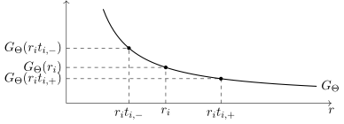
|
Figure 15. The squeeze. Only \(G_{\Theta}\) is monotone (Lemma 18.2). For lattice-rounded separations \(t_{i, \pm} \to t_{\pm}\), \(t_- < 1 < t_+\), the outer values, times \(r_i^8 \log^2 (1 / r_i)\), tend to \(A_G t_{\pm}^{- 8}\) along the radii of Lemma 18.3; letting \(t_{\pm} \to 1\) gives the limit \(A_G\). Every null sequence has such a subsequence. |
Proof of Theorem 6.18. The
phase-table reflection identity E2 of Definition 2.9 and
the reality of \(T\) in Lemma 16.18 make \(e_{\text{tr}}\)
real. Lemmas 16.17, 16.18 and 17.11
show that \(\Theta\) is real and \(O (4)\) invariant and that its
continued label is Hermitian and Lorentz scalar. Lemma 18.1
gives vacuum centering. For the asymptotic, take any prescribed positive
null sequence and the subsequence in
Translation and \(O (4)\) invariance (Lemma 17.3) give \(S_2^{\xi_{\ast}} (\Theta, \Theta ; rx_0, rx_1) = G_{\Theta} (r|x_0 - x_1 |)\). Here \(\kappa_G^{- 2} (4 d_2)^2 = 1\), so the amplitude does not depend on \(\kappa_G\).
Take \(x_0 = 0\) and \(x_1 = (t / 2, t / 2, t / 2, t / 2)\), with \(1 / 2 < t < 2\). This pair is generic and has distance \(t\). Monotonicity from Lemma 18.2 bounds the lower limit at radius \(r_i\) by \(A_G / t^8\) for \(t > 1\), and the upper limit by that expression for \(t < 1\) (Figure 15). Let \(t \to 1\). The limit along this subsequence is \(A_G\). The subsequence criterion gives the full-radius limit. Here \(A_G = 3 d_{\mathfrak{g}} / \pi^4 > 0\) since \(d_{\mathfrak{g}} \geqslant 1\); identifying it uses \(d_2 = - \kappa_G / 4 \ne 0\). Thus \(\Theta \ne 0\).\(\Box\)
The following high-energy law follows from Theorem 6.18 and Lemma 18.2, as proved below.
Lemma
Proof. The rescaled spectral measures are controlled through their Laplace transforms, which the trace law determines (Definition 6.17, Lemma 18.2). Put \(\nu_{R_{\text{E}}} = R_{\text{E}}^{- 8} \log^2 R_{\text{E}} \hspace{0.17em} \mu_{\Theta} (R_{\text{E}} \hspace{0.17em} \cdot)\). For every future timelike Laplace covector \(u\), with the Euclidean pairing \(u \cdot \mathbf{p}\) of item W0 of Definition 2.14, which is the Minkowski pairing of \(\mathbf{p}\) with the future timelike \((- u^1, - u^2, - u^3, u^4)\), Lorentz invariance reduces its transform to the time-axis transform at \(s = \sqrt{\textsf{m} (u)}\). Hence
To identify the constant, write \(t =\mathbf{p}^4\) and integrate the spatial radius \(q\):
The \(s = 1\) transform bounds compact masses, so diagonal extraction and Riesz representation [30, Theorem 2.14] give vague subsequential limits. The \(u / 2\) transform controls the \(u\)-damped tail, so every limit has the displayed transforms. Holomorphic uniqueness in each coordinate for timelike real part, then Fourier inversion on product Schwartz tests against the finite damped measures [30, Theorems 10.18 and 9.11], identify every limit with the cone density in the statement.
For Schwartz tests positivity gives
Use the trace law at \(1 / (R_{\text{E}} R)\) and \(\log R_{\text{E}} \leqslant \log (R_{\text{E}} R)\). A Schwartz bound of order greater than eight sums the dyadic energy tails uniformly, since \(|\mathbf{p}| \leqslant \sqrt{2} \mathbf{p}^4\) on the cone. The \(C_c\) limit then gives the Schwartz limit.\(\Box\)
For \(\psi_{R_{\text{E}}} (x, y) = R_{\text{E}}^8 \psi (R_{\text{E}} x, R_{\text{E}} y)\), \(\mathcal{W}_{\text{rel}} \psi_{R_{\text{E}}} (\mathbf{p}) =\mathcal{W}_{\text{rel}} \psi (\mathbf{p}/ R_{\text{E}})\). For \(\psi \in \mathcal{S}_2\), \(\mathcal{W}_{\text{rel}} \psi \in \mathcal{S}\). Substitution in Lemma 18.9 gives the position-space consequence
A finite Wick profile of Definition 2.18 is, at small distance, a finite sum of terms \(r^a \log^k r\) with \(a \in \mathbb{Z}\) and \(k \geqslant 0\), plus a bounded remainder; the trace law requires the negative logarithmic power \(\log^{- 2} (1 / r)\). This gives the following exclusion; its proof follows.
Lemma
Proof. We expand each profile at small \(r\) and compare with the positive limit of Theorem 6.18. For one factor, polar coordinates and \(\omega_{m_{\text{sh}}} = \sqrt{m_{\text{sh}}^2 + q^2}\) give
For \(m_{\text{sh}} = 0\) this is proportional to \(r^{- j_h - k_E - 2}\). Otherwise split at \(2 m_{\text{sh}}\); the bounded interval is analytic. On the tail expand \((1 - m_{\text{sh}}^2 / \omega_{m_{\text{sh}}}^2)^{(j_h + 1) / 2}\). Taking enough terms makes the remainder integrable with any prescribed number of energy moments, hence gives a Taylor remainder of the required order. The retained terms are \(I_a (r) = \int_{2 m_{\text{sh}}}^{\infty} v^a e^{- rv} \hspace{0.17em} dv\), \(a \in \mathbb{Z}\). Integrate explicitly for \(a \geqslant 0\); \(I_{- 1}' = - e^{- 2 m_{\text{sh}} r} / r\) gives the logarithm, and \(I_a' = - I_{a + 1}\) gives all lower powers. Only nonnegative logarithmic powers occur. For products, choose each remainder order above the other factors' pole orders.
Thus \(\text{Re} \hspace{0.17em} W_{\text{Wick}} = \sum_{a, k} c_{a, k} r^a \log^k r + O (1)\) with finitely many terms. After multiplying by \(r^8 \log^2 (1 / r)\), the terms with \(a > - 8\) vanish. Among the others, the least \(a\), then largest \(k\), gives a nonzero divergent leading term. A finite limit is therefore zero. Lemma 18.2 makes \(G_{\Theta}\) real, so equality with \(W_{\text{Wick}}\) implies equality with its real part. The positive trace limit contradicts equality on \((0, \delta)\), proving also Proposition 6.19.\(\Box\)
To describe polynomial mass-shell Wick contractions, put \(q_m (\mathbf{k}) = (\mathbf{k}, \sqrt{m^2 + |\mathbf{k}|^2})\), \(m \geqslant 0\). Fix a finite set of elementary field indices, with elements \(\textsf{x}, \textsf{x}'\); words \(u, u'\) list its elements. For words of length \(k\), \(\pi\) ranges over permutations of \(\{1, \ldots, k\}\). Comparison data specify finite mass–polynomial lists \(\mathcal{M}_{\text{pair}} (\textsf{x}, \textsf{x}')\), with \(P \in \mathbb{C} [\mathbf{p}^1, \ldots, \mathbf{p}^4]\), and complex contraction coefficients \(c (u, u', \pi)\).
Definition
For words \(u = (\textsf{x}_i)_{i = 1}^k\), \(u' = (\textsf{x}'_i)_{i = 1}^k\), define the convolutions of the functionals \(L_{m, P}\) by
For unequal lengths put \(\textsf{P} = 0\). A zero denominator at zero momentum gives value zero.
For finite polynomial fields \(Q = \sum_i \alpha_i u_i\), including empty words, the bilinear pairing is \(W^{\text{pol}} (Q, Q' ; \varphi) = \sum_{i, j} \alpha_i \alpha'_j \textsf{P} (u_i, u'_j ; \varphi)\). Empty contractions evaluate \(\varphi\) at zero. The shell measure has no \((2 \pi)^{- 3}\) factor.
The next lemma separates each comparison by one product test; its proof follows.
Lemma
Proof. Equality for all product tests would identify the two spectral representations, hence \(G_{\Theta}\) with a finite Wick profile, which Lemma 18.10 excludes. In detail, equality for all product tests implies equality for every \(\varphi \in C_c^{\infty}\): choose \(\hat{h}_+ = \varphi\) and real \(\hat{f}_+ = 1\) on its support. Approximate \(e^{- r\mathbf{p}^4}\) by compact cutoffs. Dominated convergence applies: Lemma 18.2 controls \(\mu_{\Theta}\); exponential damping controls comparison polynomials at infinity, and \(d^3 \mathbf{k}/ |\mathbf{k}|\) is integrable at zero. Expanding the numerators into monomials factors the integrals into the kernels of Definition 2.18, with the empty words giving constants. Hence \(G_{\Theta} (r) = W_{\text{Wick}} (r)\) for all \(r > 0\), contrary to Lemma 18.10.\(\Box\)
For the photon comparison use Hilbert tensor products.
Definition
The density vanishes at zero momentum, so the value of \(\Pi\) there is immaterial, and \(\Pi\) acts pointwise. Thus a physical vector is symmetric and transverse in each slot. Translations multiply sector \(k\) by \(\exp \{iz \cdot \sum_j (\mathbf{k}_j, |\mathbf{k}_j |)\}\). The sector-zero unit is \(\Omega_0\).
Definition
A comparison \(U : \mathcal{H} \to \mathcal{F}_n\) is a complex linear isometry with image in \(\mathcal{F}_n^{\text{phys}}\), \(U \Omega = \Omega_0\), intertwining translations. Set \(\psi_U (f) = U \Phi_{\Theta} (f) \Omega\).
Real tests have real components. Causal separation means \(\textsf{m} (x - y) < 0\) for every pair of points in their closed supports, where \(\textsf{m} (x) = (x^4)^2 - \sum_{a = 1}^3 (x^a)^2\).
Lemma 18.12 compares two-point functions only. The Fock test asks more: an embedding of the interacting states into photon Fock space under which the trace field is local relative to the free Maxwell field. Relative locality would impose the equality excluded below. Formally, let \(W (h)\) be Weyl operators of the free Maxwell field with \(W (h) \Omega_0 =\mathcal{E} (h)\) and \(W (h)^{\ast} = W (- h)\). If \(U \Phi_{\Theta} (f) U^{\ast}\) commuted with \(W (h)\) for \(h\) causally separated from \(f\), then, since \(U^{\ast} \Omega_0 = \Omega\) and \(\iota_4 \Theta\) is Hermitian,
Weyl operators enter only this motivation. The lemma compares the two matrix elements directly, and its proof uses spectral growth without restricting particle amplitudes.
Lemma
Proof. The proof combines the spectral representation (Lemma 18.2), the high-energy law (Lemma 18.9) and translation covariance (Lemma 17.5) with the dilation behaviour of local photon amplitudes. Fix a ball and suppose equality always holds.
Sector amplitudes. Set \(p_j = (\mathbf{k}_j, |\mathbf{k}_j |)\) and \(p_{\text{tot}} = \sum_j p_j\). The convolution argument of Lemma 18.2 gives sector amplitudes \(Y_{k, s}\), with \(s\) listing colour and spatial indices:
| \(\displaystyle \psi_U (f)_{k, s} = \hat{f}_+ (p_{\text{tot}}) Y_{k, s}, \qquad \mu_{\Theta} = (p_{\text{tot}})_{\ast} \sum_{k, s} |Y_{k, s} |^2 d \sigma^{\otimes k} \hspace{0.17em} .\) | (18.11) |
Box masses are finite. Cauchy–Schwarz and polynomial spectral growth give integrability against sufficiently high inverse polynomials in each momentum.
The common sector unitary \(i^k\) preserves the equality, physical vectors and translations. Write \(\textsf{Y} = i^k Y_{k, s}\).
Locality and doubling. Expand the coherent equality in a real parameter multiplying \(h\), justified by Cauchy–Schwarz and the exponential series. Polarization and complexification give independent complex slot tests. Transversality removes the projector in contractions with physical waves. Shrink nonnegative unit-integral \(f\) to zero. Then \(| \hat{f}_+ | \leqslant 1\) and \(\hat{f}_+ \to 1\); dominated convergence gives, for \(g_j\) supported spacelike to zero,
Here \(\hat{g}_- (p) = \hat{g}_+ (- p)\); the sector factors \(i^k\) give exactly these signs.
Fix other slots and use \(g (x, t) = a (x) \eta_{\epsilon}^{(b)} (t)\),
with \(\eta_{\epsilon}\) approximating unit mass and \(b = 0, 1\). If
\(0 \not\in \text{supp} \hspace{0.17em} a\), these are spacelike for
small \(\epsilon\). Thus both Cauchy data of
Each datum depends only on the \(J\)-jet: multiplication by a cutoff in \(B (0, \epsilon)\) leaves the distribution unchanged. For a zero-\(J\)-jet test, Taylor's formula bounds derivatives through order \(J\) by \(O (\epsilon)\); let \(\epsilon \downarrow 0\).
The next paragraph proves a uniqueness implication: a combination of sector amplitudes whose two Cauchy data vanish is zero almost everywhere. It is applied below to a polynomial in the doubling operator applied to \(\textsf{Y}\), not to \(\textsf{Y}\) itself. The massless wave equation separates the frequency branches from these two Cauchy data away from zero momentum. After smearing other slots, each branch is integrable, bounded and holomorphic in its timelike tube, with continuous real boundary. For such a combination with zero Cauchy data, vanishing persists under small translations of the other spacelike tests. Schwarz reflection and holomorphic uniqueness [30, Theorems 11.14 and 10.18] make the zero set invariant under adding \(\mathbb{R}u\) for every future timelike \(u\). These vectors span \(\mathbb{R}^4\), giving vanishing at every real translation. Successive Fourier inversion [30, Theorem 9.11] of the smeared integrable amplitudes gives zero almost everywhere. Countably many shrinking bumps remove the other tests: their transforms are eventually nonzero at each momentum.
Let \(D_j \textsf{Y} (\boldsymbol{k}) = \textsf{Y} (\mathbf{k}_1, \ldots, 2\mathbf{k}_j, \ldots, \mathbf{k}_k)\). In the time-order-\(b\) Cauchy datum (\(b = 0, 1\)), this substitution gives \(2^{- 3 - b}\) times the datum at \(a (x) \mapsto 8 a (2 x)\), from \(d \sigma (2\mathbf{k}) = 4 d \sigma (\mathbf{k})\) and \(|\mathbf{k}|^{1 + b}\). Spatial jets of order \(l\) scale by \(2^{3 + l}\), giving eigenvalues \(2^{l - b}\). Choose a polynomial that annihilates this finite-dimensional dilation action on both Cauchy jets. The uniqueness implication then makes the same polynomial in \(D_j\) annihilate \(\textsf{Y}\): for some \(J'\),
| \(\displaystyle \prod_{a = 0}^{J' - 1} (D_j - 2^{a - 1}) \textsf{Y} = 0 \qquad \text{in every slot } j \hspace{0.17em} .\) | (18.13) |
Growth. For \(R = 2^l\) let \(M_{\textsf{Y}} (R) =
\int_{|\mathbf{k}_j | \leqslant R} | \textsf{Y} |^2 d
\sigma^{\otimes
k}\). By
| \(\displaystyle M_{\textsf{Y}} (2^l) \leqslant \mu_{\Theta} \{\mathbf{p}^4 \leqslant (k + 1) 2^l \}, \qquad 2^{- 8 l} M_{\textsf{Y}} (2^l) \longrightarrow 0 \hspace{0.17em} .\) | (18.14) |
For the limit, bound the energy mass by \(e \hspace{0.17em} G_{\Theta} (((k + 1) 2^l)^{- 1})\).
Lagrange interpolation in the commuting \(D_j\) splits \(\textsf{Y}\)
into joint eigencomponents \(D_j \textsf{Y}_{\boldsymbol{e}} = 2^{e_j -
1} \textsf{Y}_{\boldsymbol{e}}\). Each is a finite combination of
doubled copies, so retains
Summing
An averaged form of this countertest, in which the coherent vectors are moved by maps that preserve physical inner products and fix the image of \(U\), is Lemma 8.10 in Section 8.
This section proves Theorems 6.20 and 6.21. The coefficients of the product expansion are read off by probes. A finite family of probe correlations distinguishes the fields of a fixed degree: two fields of \(F_j\) with the same correlations against every probe are equal. Applied to a cluster of insertions, the probes return finitely many numbers, and a fixed linear reconstruction map, a decoder, returns a field of \(F_j\); on the probe values of a single field it returns that field. Lower degrees are removed before the next degree is read. The probes are chosen once, before the spectators and the phase, and the coefficients are computed from the mixed table; hence they depend on the cluster alone. The remainder is bounded in the commutative compression algebra \(\mathfrak{A}_0\) of Lemma 17.1 before a character is evaluated, and a norm bound in \(\mathfrak{A}_0\) bounds every character and the mixed vacuum. The coefficients do depend on the prescription, that is, on the table and the probes chosen here; Theorem 6.20 concerns this one coefficient system.
For two fields \(A, B\) of degrees \(d_A, d_B\) at \(x\) and \(0\), with center \(0\) and \(|x| \asymp r\), the expansion tested against spectators reads
with \(|c_{j, \lambda} | \leqslant r^{j - d_A - d_B - \varepsilon}\) and \(|\mathcal{R}_D^{\zeta} | \leqslant r^{D + 1 - d_A - d_B - \varepsilon}\) for small \(r\); \(O_{0, \lambda}\) is a nonzero multiple of the unit. For \(D + 1 < d_A + d_B\) the remainder bound still permits growth as \(r \to 0\); what increases with \(D\) is its order, and once \(D \geqslant d_A + d_B\) (with \(\varepsilon < 1\)) the remainder tends to zero. Nothing is asserted about a series in \(D\). The expansion goes back to Wilson [35]; Fröb and Holland prove its existence for Euclidean Yang–Mills theory to all orders in perturbation theory [13]. The expansion here is nonperturbative, at each finite truncation, with one coefficient system for every phase.
The lattice estimate starts from the signed local and graded quotient bounds of Lemmas 19.1 and 19.2. Each insertion carries a nilpotent external field with a weight. Blocking loses mark weight when insertion points approach one another; grouping nearby markers bounds this loss by a power of the ratio of insertion and fusion scales (Figure 16). Taylor subtraction and transport of the coefficient back to a coarser level produce one field and a small remainder, whose chessboard seminorm reflection positivity converts into a norm bound in \(\mathfrak{A}_0\). Derivative induction removes the restriction to grid points; tree induction allows several clusters to shrink at independent rates. The nested and integrated forms (Lemmas 19.13–19.14 and Remark 19.15) are not used in the proofs of Theorems A and B. The contact extension of Section 19.2 is defined from the continuum correlations at distinct points, not as a lattice limit at coincident points; the lattice bounds of Lemma 19.9 make its shell sums converge.
Throughout, the lattice insertions and quotient fields are those of Definitions 2.8 and 2.12; inclusions and derivatives are those of Lemma 15.5. The rotations \(R_j (h)\) are those of Lemma 16.17. Write \(|\boldsymbol{A}|_{\deg} = \sum_i \deg A_i\) and \(\zeta \in \textsf{X} \sqcup \{ \text{mix} \}\), as in Definition 2.19.
We first establish two estimates needed when the field to be extracted varies with the cutoff. Throughout this subsection, a local marked expression has the form of Definition 14.5 and the regularity, zero radial jets and forced supports of Lemma 14.9. Write
The last quantity is the weighted remainder mass of Lemma 14.7. Fix an output degree \(t\). The diagonal rescaling \((\textsf{d}_i x)_{\alpha} = \ell_i^{t - \deg \alpha} x_{\alpha}\) accounts for the engineering degrees inside \(V_t\). Write \(C_i = C^{\text{col}}_{J_i}\) for the column bound at level \(i\). A normalized column at level \(i\) is the local expression \(\mathfrak{c}_i (b)\) of Lemma 14.7 with coefficient vector \(b\); its coefficient map is \(\textsf{C}_i\), and its remainder bound is \(C_i \mu ((\textsf{C}_i b)^{\circ})\) by Lemma 14.7.
Let \(K_j \geqslant 1\) be the nondecreasing stage bound fixed before item 1 of Section 14.1. The degree rescaling above is the map \(\textsf{S}_L\) in the proof of Lemma 14.6. For an input coefficient \(v\) and remainder mass \(q\), its averaged marked estimate gives an output coefficient \(u\) and remainder mass \(r\) with
Here \(M_i\) is the leading polynomial map, fixes the unit, preserves
the nonconstant subspace, and satisfies \(\|M_i^{\pm 1} \| \leqslant
K_{J_{i + 1}}\). These estimates follow from
The column choice imposes the first inequality; the ratio choice imposes the other two. Stage growth gives \(J_{l + 1} \leqslant J_l + 1\).
The next estimate retains the signed difference produced by subtracting a column. A transported family on \([k_{\ast}, m]\) is a sequence of local marked expressions \(\mathfrak{c}_l (x_l) + R_l\), \(k_{\ast} \leqslant l \leqslant m\), in which \(R_l\) has coefficient zero and each term arises from the next finer one by one marked integration step of Lemma 14.6; \(x_l\) are its coefficients and \(r_l\) its remainder bounds. Its free affine parameter is a vector added to the column coefficient at the finest level \(m\). Write \(q_{\text{fin}}\) for the combined coefficient and remainder bound of the original expression at \(m\), before this affine subtraction. In the next lemma, the interval \([k_{\ast}, m]\) is sufficiently late.
Lemma
(b) If \(x_{k_{\ast}} = 0\), then, for \(k_{\ast} \leqslant l \leqslant m\),
Thus a residual that starts with zero coefficient at the coarse end loses only the factor \(4 (1 + C_m)\) at the fine end, and gains \((a_m / a_l)^{1 / 8}\) at every coarser level.
Proof. The termwise remainder estimates and the Lipschitz bound in the proof of Lemma 14.6 control one step; the exact column identity of Lemma 14.7 keeps the densities exact; an induction along the interval turns the signed one-step inequalities into the discount.
Let \(R\) have coefficient zero and remainder bound \(q_0\). Its regular
terms have zero radial jets through \(t\), by the local format of Lemma
14.9; its forced terms retain their eligibility events. In
the marked integration of Lemma 14.6, the former gain an
inverse block factor before the connected sums, and the latter keep half
the forced suppression. The stage constants precede the ratio and its
entry threshold, so both resulting bounds \(C^{\text{loc}}_{J_{i + 1}} /
\ell_i + o_{\hat{\beta}_i} (1)\) are at most \(\ell_i^{- 2 / 5}\). Sum
the regular masses \(g_a\) and forced masses \(k_b / (\epsilon_{i +
1}^{\text{for}})^{1 / 2}\) before taking the output norm. Their sum is
at most \(q_0\). The termwise bounds in that proof, or its Lipschitz
estimate for the difference between a column plus \(R\) and the same
column, therefore bound the output coefficient and remainder by
\(\ell_i^{- 2 / 5} q_0\). The rooted clause of Lemma 13.5,
in the marked norm defined below, justifies termwise integration and
retains the exact density identity. The last inequality of
Write the fine affine family as \(\mathfrak{c}_{i + 1} (a + b) + R\), with \(b\) the free parameter. Set \(c = \textsf{C}_i^{- 1} z\) and replace it at the coarse level by
The coefficient of \(R'\) is zero, and \(\mathfrak{r}_i (R') \leqslant (1 + C_i) \ell_i^{- 2 / 5} q_0\). Linearity of the column density gives \(H (\mathfrak{c}_i (a + c + b)) + H (R') = H (\mathfrak{c}_i (a + b)) + H (Z)\). Together with the exact column identity of Lemma 14.7, this proves the asserted density identity for every \(b\), including all forced terms. The supports remain fixed in \(b\) by Lemma 14.7.
For the column alone use
For later use put \(U = \mu (u)\), \(Y = \mu (\textsf{d}_i v)\), \(K = K_{J_{i + 1}}\) and retain \(r, q\) for the remainder bounds. Applying \(M_i^{- 1}\) and using \(\mu (v^{\circ}) \leqslant Y\) gives
| \(\displaystyle Y \leqslant K [U + \epsilon_i (Y + q)], \qquad r \leqslant KY + \epsilon_i q \hspace{0.17em} .\) | (19.3) |
For an interval \([k_{\ast}, m]\), choose the free affine parameter to
cancel the coefficient at \(k_{\ast}\); this uses the invertibility of
\(\textsf{C}_{k_{\ast}}\). The signed residual then starts with
coefficient zero. In step \(l\) put \(K = K_{J_{l + 1}}\) and \(A_l = 32
(1 + C_l)^2\). Induct from \(k_{\ast}\) toward \(m\) on the cone
condition \(A_l \mu (x_l) \leqslant r_l\), which says that the
coefficient is small compared with the remainder bound; it holds at
\(k_{\ast}\) because \(x_{k_{\ast}} = 0\). Equation
In
The next estimate recovers the output-degree power after passing to the
quotient. Fix any norm on \(F_t\). Put \(\|v\|_m = \mu (x_m (v))\),
where \(x_m (v) = x_{N, p, m ; t} (v)\) is the transferred coefficient
of Definition 2.8. A refinement below is a nontrivial
refinement of the ordered cutoff limits
Lemma
| \(\displaystyle \text{dist}_{F_t} ([v], \jmath_{i - 1, t} F_{i - 1}) \leqslant C_{t, i} (m) a_m^{- (t - i)} \epsilon_{\text{bd}} \hspace{0.17em} .\) | (19.4) |
Here \([v] \in F_t\) is the class of \(v\), \(F_{- 1} = 0\), and \(m\) is sufficiently large.
A label that is small at level \(m\) is therefore, in the quotient and up to subpower factors, within \(a_m^{- (t - i)}\) times its size of the fields of degree below \(i\).
Proof. The triangularity of the
leading map proved in Lemma 14.6 separates high from low
engineering degrees; the marked bounds of Lemma 14.7
control the error; the physical quotient of Definition 2.12,
with the corrected inclusions of Lemma 15.5, identifies the
removed low-degree part with a lower field. In the notation of
The diagonal entries are the nonzero fine-to-coarse normalization factors. The full coefficient map differs from this leading map by the marked error. Write \(P\) for coordinate projection onto engineering degrees at most \(i - 1\), first assuming \(i > 0\). The leading map \(M_l\) and its inverse preserve \(\ker P\): triangularity gives preservation by \(M_l\), and injectivity on this finite-dimensional subspace gives preservation by its inverse. Consequently \(\mu (Px) \leqslant K_{J_{l + 1}} \mu (PM_l x)\). The degree rescaling expands \(Px\) by at least \(\ell_l^{t - i + 1}\), whereas it expands \(x - Px\) by at most \(\ell_l^{t - i}\). The marked error is bounded by \(\epsilon_l \mu (x^{\circ})\).
The two resulting estimates are
To obtain the first line, put \(Y = \mu (P \textsf{d}_l x_{l + 1})\).
The low-cone hypothesis \(\mu (x_{l + 1}) \leqslant C_{l + 1} \mu (Px_{l
+ 1})\) and \(C_{l + 1} \leqslant \ell_l\) give \(\mu (\textsf{d}_l x_{l
+ 1}) \leqslant 2 Y\). Applying the inverse leading map to the low
coordinates and using \(2 K_{J_{l + 1}} \epsilon_l (1 + C_{l + 1})
\leqslant 1\) gives \(Y \leqslant 2 K_{J_{l + 1}} \mu (Px_l)\). The full
coefficient is at most \(3 K_{J_{l + 1}} Y\), so \(64 K_{J_{l + 1}}^2
\leqslant C_l, C_{l + 1}\) gives both conclusions. In the second line
use \(\mu (\textsf{d}_l x_{l + 1}) \leqslant \ell_l^{t - i} \mu (x_{l +
1})\) and \(K_{J_{l + 1}} + 1 \leqslant C_{l + 1}\). These numerical
inequalities follow from
At the bare level take the plane \(PV_t\). Its transported image remains in the low cone by the first line. The map from this plane to its low coordinates at any level is injective by its expansion bound, hence onto \(PV_t\). Subtracting a transported vector with the same low coordinates at level \(m\) therefore leaves zero low coordinates and increases the full size by at most \(1 + C_m\). Repeat the subtraction at every next coarser level, applying the second line between subtractions. This gives a vector \(y_{N, p}\) in the transported bare low plane with
Allowing a fixed norm-equivalence factor, put \(\mathcal{J}_m = \prod_{l < m} C_{l + 1}\). The first-line expansion, iterated from the bare level, shows that bounded vectors \(y_{N, p}\) in this plane have bare coefficients bounded by \(a_N^{t - i + 1} e^{o (s_N)}\). Multiplying the same polynomial by \(a_N^{i - 1}\) instead of \(a_N^t\) therefore gives a degree-\((i - 1)\) local observable with subpower healthy derivative and all-configuration supremum bounds. Its stencil is unchanged. To match this observable to the selected lower-degree insertions, apply Lemma 14.17(i): it gives tame degree-\((i - 1)\) coefficients \(c_{N, p}\) whose insertions differ from these observables by a negligible error (Definition 14.16). Lemma 15.3 removes that error in every separated spectator test.
To pass to a physical lower field, apply Lemma 15.4 in
\(V_{i - 1}\) to the family \(c_{N, p}\), with the equation projections
\(\Pi_{N, p} = \Pi_{i - 1, N, p}\) of Lemma 14.18, taken
along \(N = \textsf{n} (j)\) and \(p = P (k)\), their limit \(\Pi_{i -
1}\) from
For \(i = 0\) no plane is removed. Iterating the reverse coefficient estimate of Lemma 14.7 gives \(\|v\| \leqslant \mathcal{J}_m (a_{m_{\text{ref}} (t)} / a_m)^t \epsilon_{\text{bd}}\) and hence the same bound in \(F_t\). Finally \(\log \mathcal{J}_m = o (s_m)\), since \(\log C^{\text{col}}_{J_{m + 1}} \leqslant J_{m + 1}^{- 2} \log \ell_m\) (Section 9) and by Lemma 14.2. Since \(C_l \geqslant 2\), \(G_m C_m \leqslant (\mathcal{J}_m)^3 C_0\). Thus \(\log G_m = o (s_m)\) as well. Fixed reference-spacing and quotient-norm factors are absorbed in \(C_{t, i} (m)\). No estimate depends on the refinement used to take the limits.\(\Box\)
A probe word is a fixed finite list of fields at distinct nonzero points. Correlating a field at the origin against such a word gives a linear functional on \(F_j\). The intersection of the kernels of all these functionals is zero, by the definition of \(\mathcal{N}_j\). Finite dimensionality therefore permits a finite separating collection.
Choose the probe functionals recursively. Given biorthogonal fields \(u_{\alpha}\) and probe functionals \(\ell_{\alpha}\) below degree \(j\), continue each \(\ell_{\alpha}\) to \(F_j\) by the same correlation formula; inclusions preserve that formula by Lemma 15.5. The retraction
allows a section \(s\) of the new quotient to be replaced by \(s - \jmath \textsf{t}_j s\). Lift a quotient basis with this section and realize its dual by finite combinations of probe functionals, which span \(F_j^{\ast}\). The enlarged system is biorthogonal. In particular \(\ell_{\alpha}\) vanishes on \(\jmath F_{\deg \alpha - 1}\). For \(j = 0\) take \(u_0 =\boldsymbol{1}\). Let \(\mathcal{P}_j\) be the union of the finite probe sets used through degree \(j\), with index \(\gamma\). Write \(\ell_{\alpha} (A) = \sum_{\gamma} m_{\alpha \gamma} S (A (0), B_{j, \gamma})\) in this finite collection.
Definition
With \(\text{ev}_j (A) = (S (A (0), B_{j, \gamma}))_{\gamma \in \mathcal{P}_j}\), it satisfies \(D_j \text{ev}_j = \text{id}_{F_j}\): it is a fixed left inverse of field evaluation. For a word \(w\) separated from these probes, set
This extracts a field from finitely many correlations using the fixed biorthogonal coordinates.
Here and below a word is a finite product of labelled insertions; sums of words are read linearly. Rotations act on every position and label, and conjugation acts on labels and scalar coefficients. Translation of a word by \(u\) is denoted by \(\tau_u\).
Definition
The Haar measure has mass one. Outside this domain set both maps to zero. At center \(o\), apply these formulas to \(\tau_{- o} w\). These averages impose rotation covariance and reality.
Let \(I_q A = A (0)\) for \(A \in F_q\). The inclusions \(\jmath_{i, j}\) identify the same field in different degrees.
Definition
For the chosen real basis \((O_{j, \lambda})_{\lambda \in \text{Ch}_j}\) of \(E_j\), let \(\omega_{j, \lambda} : E_j \to \mathbb{C}\) be its coordinate functionals and set
The recursion removes lower degrees before reading coordinates and is independent of arity and truncation.
In the first two degrees the recursion reads as follows. In degree zero, \(Q_0 = 1\): the degree-zero probes read the multiple of the unit line seen by the cluster. In degree one, \(L_{0, 1} = B_0 I_1\) reads the degree-zero part of a single degree-one field, and
This is the field read in degree one, minus the multiple of the unit that the degree-zero probes see in it. The degree-one coefficients are the coordinates of this difference in \(E_1 = \ker L_{0, 1}\).
The following splitting makes the coefficients a single choice for all later estimates.
Lemma
The degree-zero vector spans the unit line and need not equal the unit.
By Definition 19.5, all coefficients are fixed before spectators, states and truncations.
Proof. The biorthogonal construction preceding Definition 19.3 gives a reconstruction formula fixing every field of \(F_j\); the field calculus of Lemma 15.5 makes the old functionals compatible with the inclusions. Continuing an old functional means using the same finite correlations, since \(\iota_j \jmath_{q, j} = \iota_q\); no extension of a functional is chosen arbitrarily.
For \(i \geqslant q\), this reconstruction and the rotation and reality laws give \(L_{i, q} = \jmath_{q, i}\). Also \(L_{i, j} \jmath_{q, j} = L_{i, q}\) for \(i < q \leqslant j\): both sides evaluate the same single-field word before averaging. For all \(q \leqslant j\), induction in \(j\) now gives
| \(\displaystyle Q_j L_{j, q} = 0 (q < j), \qquad \sum_{i \leqslant j} \jmath_{i, j} Q_i L_{i, q} = \jmath_{q, j} \hspace{0.17em} .\) | (19.5) |
For \(q = j\) the second identity is the recursion; for \(q < j\),
compose that recursion with \(\jmath_{q, j}\) and use the compatibility
just proved and the induction hypothesis. In the same induction assume
\(Q_k F_k \subset E_k\) and \(Q_k = 1\) on \(E_k\) for \(k < j\).
Applying \(Q_i L_{i, j}\) to \(Q_j A\) then cancels its matching \(i\)
term; terms with \(k < i\) vanish because \(Q_i L_{i, j}\) vanishes on
\(\jmath_{i - 1, j} F_{i - 1}\), and terms with \(i < k < j\) vanish
because \(Q_k A \in E_k\). Thus \(Q_j F_j \subset E_j\). On \(E_j\), the
defining sum for \(Q_j\) is zero, so \(Q_j = 1\). Its kernel is exactly
\(\jmath F_{j - 1}\) by
For \(T \to \infty\) write \(f \preccurlyeq e^{bT}\) when, for every \(\tau > 0\), there is \(T_0\) such that for every \(T \geqslant T_0\) an ordered cutoff tail gives \(\|f\| \leqslant e^{(b + \tau) T}\), uniformly in the cutoff and volume on that tail. Products add exponents and finite sums take their maximum. Factors of exponent zero are called subpower. A level \(k\) has height \(b\) when \(s_k / T \to b\); thus \(a_k = e^{- bT + o (T)}\). Lemma 14.2 supplies these levels by taking the first with \(s_k \geqslant bT\), or \(s_k \geqslant \sqrt{T}\) if \(b = 0\).
Insertions are carried through the integration by nilpotent external fields. This is the device used for observables by Bauerschmidt, Brydges and Slade, who add an external observable field to the interaction and truncate the algebra in it [5, Section 2.3]. A marker is one group of insertions in the reflected cells not yet fused with another; it is live while its weight is positive. To each marker \(\iota\) attach a commuting variable \(z_{\iota}\) with \(z_{\iota}^2 = 0\) and a mark weight \(w_{\iota} > 0\). In this finite scalar algebra put
Products of monomials with overlapping markers vanish, and the weights of disjoint markers multiply, so \(\|cd\|_{\text{mark}} \leqslant \|c\|_{\text{mark}} \|d\|_{\text{mark}}\). The coefficient of \(z_A\) in \(\rho \prod_{\iota} (1 + z_{\iota} O_{\iota})\) is \(\rho \prod_{\iota \in A} O_{\iota}\); by linearity, taking this coefficient commutes with integration of integrable terms.
If \(F_{X, A}\) is a coefficient with support \(X\) and marker set \(A\), its weighted majorant is
Here \(\|F_{X, A} \|\) is the derivative or forced majorant of Definitions 5.3–5.4; at a support ball use its anchored sum. The factors \(e^{\sigma \text{cov} (X)} \|F_{X, A} \|\) enter as \(v_a\) in Lemma 13.5. Only the marked norm is used submultiplicatively. A grouped coefficient carries the product of its live mark weights, denoted by \(\omega\).
For the marked expansion put
The fixed integer \(\nu_t\) bounds the local degree-\(t\) polynomial losses, and \(y_{t, l} C_l \leqslant 1\) at entry. The four factors pay respectively for support enlargement, regular transport, Taylor extraction and insertion normalization. Their logarithms and \(\log C_l\) are \(o (s_l)\). For an initial weight \(\varpi > 0\) at \(k_{\ast}\) define its later weights by
The marked entry choices require \(\phi_l \ell_l^{t + 1} y_{t, l} \leqslant y_{t, l + 1}\) for \(l \geqslant m_{\text{ref}} (t)\). This follows the zero-jet regular remainder through the integration.
Let \(B_l\) be the support radius and \(q_l\) the per-site logarithmic
bound
These quantities ensure that the marked stencils fit in the cell and bound its density normalization.
For a grouped coefficient at level \(m + 1\) of weight \(\omega > 0\), put
The terminal weight \(\varpi\) must satisfy
These conditions pay for extraction at \(m\) and for the transported residual, respectively.
Informally, after blocking down to level \(m\), a group of insertions of total weight \(\omega\) is replaced by one degree-\(t\) insertion at the origin, the matched field. The next lemma bounds its coefficient by \(2\mathfrak{E}_m\), and the chessboard seminorm of the replacement error in a level-\(k\) cell by \(2 N_k / \varpi\).
Lemma
Proof. The extraction is a Taylor
expansion in the norms of Definitions 5.3–5.4
and 2.8; Lemma 19.1 transports its residual to
\(k_{\ast}\); the majorants of Lemma 13.12, summed by the
rooted clause of Lemma 13.5 in the marked norm, bound the
cell integral. Divide a grouped coefficient by its available weight
\(\omega\). Extract its radial polynomial through \(t\) and write the
regular complement by the integral Taylor formula. The finite derivative
sums, coefficient conversion and remainder constants are at most
\(\Xi_m\) after the entry levels have been chosen: their logarithms are
bounded by stage constants and powers of \(\log \hat{\beta}_{m + 1}\),
whereas \(\log \Xi_m = \sqrt{\hat{\beta}_{m + 1}}\). Multiplication by
\(a_{m + 1}^t\) gives \(q^{\text{ext}}_m\). The factor four bounds the
polynomial and complement separately. Forced terms keep their original
majorants and the forced normalization in
The combined cost is at most \(2 q^{\text{ext}}_m\). Subtract the column matching the transported family at \(k_{\ast}\). Lemma 19.1 gives, for \(k_{\ast} \leqslant l \leqslant m\),
The factor \(4 (1 + C_m)\) multiplying \(2 q^{\text{ext}}_m\) includes
the finest residual and coefficient together. The entry requirement
\(\phi_l \ell_l^{t + 1} y_{t, l} \leqslant y_{t, l + 1}\) gives the
regular zero-jet gain: iterating \(\varpi_{l + 1} = \phi_l \varpi_l\)
yields \(\varpi_m \leqslant \varpi (a_m / a_{k_{\ast}})^{t + 1} y_{t, m}
/ y_{t,
k_{\ast}}\). The first condition of
In the nilpotent variables defined above, a marked polynomial is
measured by the sum of the absolute coefficients times the product of
their assigned weights. Consequently the coefficient with one residual
per cell is at most \(\varpi^{- 1}\) per cell times that sum. Summing
the unmarked majorants and dividing by the two positive density
normalizations bounds the integral per cell by \(N_k\). The singleton,
forced-profile, connected regular and eligible forced sums contribute at
most \(2, 1, 1, 1\) per cell, giving the additive constant five. Apply
this to the original local difference and the correction representing
its column, and use the triangle inequality for the chessboard seminorm,
obtained by expanding the reflected product and applying
To verify that \(k_{\ast}\) has the required height, let \(\mathfrak{n}_l = \max (1, q_l)\) bound the normalization cost. The entry choices satisfy
| \(\displaystyle B_{l + 1}^2 \leqslant 2 B_l^2, \qquad (\ell_l B_l^2)^4 \mathfrak{n}_{l + 1} = o (s_{l + 1}) .\) | (19.7) |
The level \(k_{\ast}\) exists since \(a_l B_l^2\) decreases by at least \(2 / 3\) at each step. If \(k_{\ast} = k\), the spacing ratio is one. Otherwise \(k_{\ast} = l + 1\), and minimality gives \(a_k / a_{k_{\ast}} \leqslant \ell_l B_l^2\). Therefore \((a_k / a_{k_{\ast}})^4 q_{k_{\ast}} = o (s_{k_{\ast}})\). Also \(0 \leqslant s_{k_{\ast}} - s_k = \log (a_k / a_{k_{\ast}}) \leqslant (a_k / a_{k_{\ast}})^4 \mathfrak{n}_{k_{\ast}} = o (s_{k_{\ast}})\). This proves \(s_{k_{\ast}} / s_k \to 1\) and \(\log N_k = o (s_{k_{\ast}})\). At height zero it still gives \(\log N_k = o (T)\). Finally \(\log \Xi_m = o (s_m)\) follows from \(\hat{\beta}_m = \bar{\beta} + \kappa_G s_m\) and \(s_{m + 1} / s_m \to 1\). The other displayed functions are fixed powers of \(\hat{\beta}\) or the subpower column cost of Lemma 14.2.\(\Box\)
Fix nonempty lattice labels \(v_{\iota} \in V_{d_{\iota}}\), let
\(n_{\text{cl}}\) be their number and put \(W = \sum_{\iota}
d_{\iota}\). Choose levels \(k, m, j\) of heights \(0 \leqslant \theta_-
< \theta < \theta_+\). The input points lie on the spacing-\(a_j\) grid,
in the centered level-\((m + 1)\) block \([- a_{m + 1} / 2, a_{m + 1} /
2)^4\), and their separation is at least \(B_j^2 a_j\). The
configurations belong to \(\text{Gen}_{n_{\text{cl}}}\), and all
stencils are interior to the level-\(k\) cell. These conditions hold
eventually for clusters of extent \(e^{- xT + o (T)}\) and reciprocal
separation at most \(e^{xT + o (T)}\), where \(\theta < x < \theta_+\).
The chosen \(k_{\ast}\) has height \(\theta_-\) by
Two contributions make up the exponential cost of bringing the cluster to level \(m\). The initial field normalization contributes \(W \theta_+\). Transporting at most \(n_{\text{cl}}\) groups from height \(\theta_+\) to height \(\theta\), at four powers of the scale ratio per group, contributes \(4 n_{\text{cl}} (\theta_+ - \theta)\). We therefore set
The support enlargements and the finitely many fusions contribute only subpower factors. Figure 16 shows the three scales and these costs.
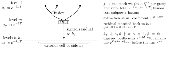
|
Figure 16. The three scales of Lemma 19.8. Markers start at the insertion resolution \(a_j\), are grouped when they cease to be \(B_l^2\)-separated, and reach level \(m\) as one group, where one degree-\(t\) field is extracted; the signed residual is matched backward to \(k_{\ast}\). Right: losses and gains up to subpower factors, at fixed truncation (no series in \(D\)). |
Lemma
The difference is interior. The bounds are uniform in cutoff and volume on that tail.
Proof. The insertions are expanded in the marked format of Definition 14.5 and Lemmas 14.7–14.9; Lemmas 19.1 and 19.7 supply the extraction once the markers form one group, and the steps below bound the mark weight lost before that. In the nilpotent variables defined above, the coefficient of their product in \(\text{dens} \hspace{0.17em} \rho_N \prod_{\iota} (1 + z_{\iota} O_{N, p} (v_{\iota}, x_{\iota}))\) is the product insertion times the density. Until level \(j\) the stencils are disjoint, so their marked integrations are separate.
Moving a marker to its representative through at most \(h\) cover balls gives
| \(\displaystyle \text{cov} (X \cup \{y_{\iota} : \iota \in A\}) \leqslant \text{cov} (X) + h |A| .\) | (19.8) |
If at most \(\mathfrak{N}\) representatives occupy a ball, shrinking each affected weight by \(\eta e^{- \sigma h}\) gives the original term times \(\eta^{|A|}\). In the anchored sum, terms incident on the old ball use its original majorant; any new incidence can be assigned to an old marker on the joining path. There are at most \(n_{\text{cl}}\) old markers for each new representative and \(\mathfrak{N}\) representatives. Taking \(\eta \leqslant [(1 +\mathfrak{N}) n_{\text{cl}}]^{- 1}\) pays for these assignments. Unmarked terms keep their supports. Hence the enlarged weighted series is bounded by the original majorant series of Lemma 13.12.
Keep a maximal \(B_l^2\)-separated set of representatives at each level, retaining the distinguished one at the origin, and attach each discarded point to a retained neighbor. A fusion decreases the number of groups, so there are at most \(n_{\text{cl}} - 1\) fusions. The joining-cover bound can be taken as \(h_l = 16 [1 + \ell_l (B_l + B_{l + 1} + 1)^2]^4\). The entry requirements of Section 9 and Lemma 14.2 give \((\sigma_{J_{l + 1}} + 1) h_l = o (s_l)\) and subpower occupancy. Choose one \(\alpha_j \leqslant 1\) below all the resulting enlargement allowances for \(m \leqslant l < j\). It is subpower: the logarithm of the running minimum is bounded by the maximum logarithmic cost; split this maximum into a fixed initial segment and a tail bounded by \(\tau s_j\), then send \(\tau\) to zero. The factor \([(1 +\mathfrak{N}) n_{\text{cl}}]^{- 1}\) above is included in this allowance \(\alpha_j / 8\).
Between fusions the one-mark integration costs at most \(6 \ell_l \leqslant \ell_l^4\) in each weight. To derive this bound, let \(\mathfrak{m}\) be an incoming marked majorant. Apply the rooted clause of Lemma 13.5 coefficientwise in the submultiplicative marked norm, with the marked factor fixed. Separate the transported regular terms into the zero-jet local integration remainder, of total weighted mass \(p_l\), and the incoming regular contribution carried without Taylor subtraction.
Use the support conversion factor \(\mathcal{A}_l\) defined by
Exponentiating bounds this incoming mass by \(\mathcal{A}_l \mathfrak{m}\); the remaining half of the fine exponent is nonnegative. Item 2 of Section 14.1 imposes \(\mathcal{A}_l \leqslant \ell_l\).
The combined regular mass is thus at most \(p_l +\mathcal{A}_l
\mathfrak{m}\). Splitting a complex marked term into its real and
imaginary parts costs at most twice its majorant. For the forced terms,
let \(f_l\) denote their total contribution after this splitting and the
normalization in
With \(g\) groups remaining, their product weight at level \(l\) is consequently at least
| \(\displaystyle (a_j / a_l)^{4 n_{\text{cl}}} (\alpha_j / 8)^{n_{\text{cl}} (n_{\text{cl}} - g)} \prod_{\iota} w_{\iota} .\) | (19.9) |
Indeed a separated step multiplies the weight by \(\ell_l^{- 4 g} \geqslant \ell_l^{- 4 n_{\text{cl}}}\). A fusion to \(g' < g\) uses at most \(n_{\text{cl}}\) factors \(\alpha_j / 8\), whereas \(n_{\text{cl}} (g - g') \geqslant n_{\text{cl}}\).
At \(m + 1\) all representatives have the same ancestor. The initial
normalized-field weights can be chosen with \(\prod_{\iota} w_{\iota} =
e^{- W \theta_+ T + o (T)}\) by Lemma 14.7. Thus
| \(\displaystyle \varpi = \exp \{[(t + 1 / 16) (\theta - \theta_-) -\mathcal{Z}] T\} .\) | (19.10) |
The second condition of
We next state the bounds when the exterior distances also shrink. Write \(w = \prod_i A_i (x_i)\), \(W = |\boldsymbol{A}|_{\deg}\) and \(V = |\boldsymbol{B}|_{\deg}\). Consider families of configurations indexed by \(T \to \infty\). Suppose the cluster lies within \(e^{- \alpha T + o (T)}\) of \(o\), its pairwise distances are at least \(e^{- \alpha T - o (T)}\), and \(\alpha > 0\). Exterior points are at distance at least \(e^{- \beta T - o (T)}\) from every cluster point and \(o\), and mutually at least \(e^{- \upsilon T - o (T)}\) apart, where \(0 \leqslant \beta < \alpha\) and \(\upsilon \geqslant \beta\). The field lists are fixed, or range over fixed compact sets of coefficients. Call these conditions (G). Let \(u_{(i, \kappa)}\), \(\kappa\) ranging over the degree-\(i\) basis fields, be the biorthogonal fields of Section 19.1, and put \(w_o = \tau_{- o} w\). Set
Here \(P_h^{\text{raw}}\) is the projection of Definition 19.3, and \(M^0\) is the compression of Definition 6.12 and Lemma 17.1.
The following estimates retain the exterior distance powers needed for nested clusters and contacts.
Lemma
The final coefficients and tested remainder of Definition 19.5 obey the same respective bounds, in norm before state evaluation.
A degree-\(i\) coordinate thus costs the cluster degree less \(i\) at the cluster height \(\alpha\), and the remainder gains \((D + 1) (\alpha - \beta)\) from the difference of the cluster and exterior heights.
Proof. The proof converts chessboard seminorms into algebra norms by Lemma 17.2, applies Lemma 19.8 on grid configurations, removes the grid restriction by derivative descent with the calculus of Lemma 15.5, and then averages the reconstruction map. Write \(n_{\text{cl}} = |I_{\text{cl}} |\).
Step 1: chessboard seminorms bound algebra norms. Suppose a lattice difference has centered chessboard seminorm (Lemma 14.15) at most \(B_{\text{rt}}\), and the exterior insertions have chessboard seminorms at most \(B_{\text{rt}, l}\). Put the difference in a coarse cell and the exterior insertions in finer disjoint cells; their stencils fit by Lemma 14.11. Let \(U \in \mathfrak{A}_0\) be the corresponding compressed difference. The lattice paragraph after Lemma 17.2, with the moment identity of Lemma 17.1, gives for every \(n \in \mathbb{N}\)
| \(\displaystyle \int_{\textsf{X}} | \xi (U) |^{2 n} \hspace{0.17em} d \nu (\xi) \leqslant (B_{\text{rt}} \prod_l B_{\text{rt}, l})^{2 n} \hspace{0.17em},\) | (19.13) |
and Lemma 17.2 gives \(\|U\| \leqslant B_{\text{rt}} \prod_l B_{\text{rt}, l}\). The same argument bounds a word by the chessboard seminorms of its insertions, giving the crude exponent \(W \alpha + V \upsilon\) on the stated geometries.
Step 2: grid configurations. Consider the generic grid configurations defined above in a cluster of height \(\alpha > 0\). Choose \(0 < \theta_- < \theta < \alpha < \theta_+\), with exterior distance exponent \(\beta < \theta_-\), and \(\mathcal{Z}= W \theta_+ + 4 n_{\text{cl}} (\theta_+ - \theta)\). Apply Lemma 19.8 with an auxiliary degree \(t \geqslant D\). For each fixed cluster geometry the output coefficients are bounded at fixed \(m\); the reverse transfer inequality of Lemma 14.7 bounds them also at the reference level. Along a refinement of the ordered cutoff tails they converge to a field \(A^{\text{out}} \in F_t\). Step 1 bounds the replacement error by exponent
Testing the same difference against the fixed probes bounds the raw
coordinate errors. Reference-level coefficient convergence and Lemma 19.2 apply on this geometry-dependent refinement. The
degree-\(i\) raw coordinate annihilates \(F_{i - 1}\) by the
biorthogonality before Definition 19.3, and is a fixed
bounded functional on the quotient. With \(\epsilon_{\text{bd}}
\preccurlyeq e^{(\mathcal{Z}- t \theta) T}\),
Choose \(t\) large enough that \((t + 1 / 16) (\theta - \theta_-) \geqslant (D + 1) \theta\) and also large enough for every coefficient being tested. Exact reconstruction of \(A^{\text{out}}\) by the prescription separates the degrees \(i \leqslant D\) from \(D < i \leqslant t\). An omitted degree contributes at most
The low-degree coordinate errors satisfy the same bound, by the chosen auxiliary horizon. We have therefore proved grid exponents \(\mathcal{Z}- i \theta\) for raw degree-\(i\) coordinates and \(\mathcal{Z}- (D + 1) (\theta - \beta) + V \upsilon\) for the raw remainder.
Step 3: derivative descent. Run the crude, grid and derivative bounds uniformly over all characters \(\xi \in \textsf{X}\). The algebra \(\mathfrak{A}_0\) is commutative, so \(\|U\| = \sup_{\xi} | \xi (U) |\). To remove the grid restriction, consider these character evaluations for every input label list and every positional derivative. A derivative replaces its input label by a field of degree one higher, by Lemma 15.5. For suitable constants \(c_0, d_0\) independent of the input degrees, the crude bound has exponent \(\alpha W + c_0\) and the grid bound exponent \(\theta_+ W + d_0\). We descend in the total input degree \(W\). The crude bound proves the desired estimate for all \(W\) with \((\theta_+ - \alpha) W \geqslant c_0 - d_0\), because \(\theta_+ > \alpha\). For the induction step, move the configuration to a generic level-\(j\) grid configuration a distance \(O (a_j)\) away; the intervening segment remains separated at exponent \(\alpha\). A positional derivative has total degree \(W + 1\), so the induction hypothesis and the grid spacing give \(e^{[\theta_+ (W + 1) + d_0] T + o (T)} a_j = e^{(\theta_+ W + d_0) T + o (T)}\): the displacement error has exactly the required degree-\(W\) bound, for every slot and axis.
Step 4: limits. Now let \(\theta \uparrow \alpha\) and
\(\theta_+ \downarrow \alpha\), keeping \(\beta < \theta_- < \theta\).
Translation moves the origin to \(o\). This proves
Step 5: the coefficients of Definition 19.5. Let
\(A^{\text{raw}}_h \in F_h\) be the raw truncation at an auxiliary
degree \(h\). In every rotated probe correlation, the difference between
the cluster and \(A^{\text{raw}}_h (0)\) has exponent \((W - h - 1)
\alpha\). The marked norm bounds and multilinearity make
At fixed exterior distances the power-separated estimates become the bounds of Theorem 6.20. The parameters \(M_{\text{geo}}\) are nonnegative and the separation and error parameters are positive, as in Definition 2.19. For the algebra-valued remainder put
Here \(M^0\) is the compression of separated words of Definition 6.12 and Lemma 17.1; its characters and vacuum state give the phase and mixed remainders \(\mathcal{R}_D^{\zeta}\) of Definition 2.19.
Lemma
Proof. Apply Lemma 19.9 to Definition 2.19, with \(T = - \log r\), \(\alpha = 1\) and \(\beta = \upsilon = 0\). Every admissible configuration has these bounds on extent and reciprocal distances. If the claimed threshold failed, choose violating configurations at radii tending to zero. The estimate just proved along that sequence, with loss \(\varepsilon / 2\), eventually contradicts the violation with loss \(\varepsilon\): constants and subpower factors are absorbed by \(r^{\varepsilon / 2}\). Taking \(M_{\text{geo}} r < \delta_{\text{sp}} / 2\) also ensures separation.\(\Box\)
Proof of Theorem 6.20. Lemma 19.6 fixes the fields and coefficients of Definition 2.19 before spectators, state indices or truncation. The coefficient bound follows from the coefficient estimate of Lemma 19.9 by the contradiction argument in the proof of Lemma 19.10; its threshold depends only on the data of the coefficient. Character evaluation and the mixed vacuum are contractions on \(\mathfrak{A}_0\), so Lemma 19.10 gives the remainder bound with its own threshold. The argument bounds \(\mathcal{R}_D\) in \(\mathfrak{A}_0\) before state evaluation.\(\Box\)
A nested configuration retains leaf positions and internal centers, so it also describes partially replaced words. Call an internal vertex other than the root proper, and fix its truncation \(D_v \in \mathbb{N}\).
Definition
Spectators are \(\delta_{\text{sp}}\)-clear of every tree position and each other.
The recursion retains every leaf, including those above a neighboring truncation.
Definition
multiplying their coefficients and summing. At the root retain only \((q, \lambda)\), giving \(C^{\text{it}, \boldsymbol{D}}_{q, \lambda}\). The direct coefficient is \(C^{\text{dir}}_{q, \lambda} = c_{q, \lambda} (\boldsymbol{A}; z_{\text{leaves}}, z_{o_{\text{root}}})\). This compares successive and direct expansion.
For example, let a cluster \(v\) of leaves of total degree \(W_v\) first fuse at scale \(\varrho_v\), and let its output then fuse with the remaining leaves at the root scale \(r\). If \(v\) is the only proper internal vertex, then
The first factor is the size allowed for the direct coefficient; the second is the truncation gain at the inner fusion. For a general tree the errors from different vertices are added, as in the definition of \(\textsf{e}_{\boldsymbol{D}}\).
Fix the tree, leaf list, output \((q, \lambda)\), proper-vertex truncations, \(M_{\text{geo}} \geqslant 0\) and \(\eta, \varepsilon > 0\). No lower bound on the ratios \(q_v\) is imposed.
Lemma
Both expressions are smooth in neighborhoods of these geometries.
Proof. The estimates of Lemma 19.9 are applied vertex by vertex along a tree induction, after reducing to sequences whose scales have convergent logarithmic heights. Along any sequence of admissible radii and scales tending to the root collision, put \(T = \sum_{v \text{ internal}} \log (1 / \varrho_v)\). Eventually every summand is positive. After a subsequence, \(\log (1 / \varrho_v) / T \to a_v \geqslant 0\), with \(\sum_v a_v = 1\) and \(a_v \geqslant a_{\text{par} (v)}\). Set
We prove by induction on the tree that a direct output of degree \(q\) has exponent \(\mathcal{B}- qa_{o_{\text{root}}}\), and its error against the prescribed finite iteration has that exponent minus \(\gamma = \min_{v \ne o_{\text{root}} \text{ internal}} (D_v + 1) (a_v - a_{\text{par} (v)})\). With no proper internal vertices the two coefficients coincide exactly.
First flatten the edges \(u \to v\) with \(a_u = a_v\): combine their
grouping before making any field replacement. The word at \(v\) then
consists of original leaves in this equal-height component and outputs
from strictly finer children; its distinct positions are separated at
exponent \(a_v\) by the tree geometry. For a child with \(a_u > a_v\),
expand to an auxiliary horizon \(H_u\). The remainder exponent has the
improvement \((H_u + 1) (a_u - a_v)\) by
| \(\displaystyle \prod_{i = 1}^n X_i - \prod_{i = 1}^n Y_i = \sum_{i = 1}^n \left( \prod_{h < i} Y_h \right) (X_i - Y_i) \left( \prod_{h > i} X_h \right)\) | (19.14) |
justifies these successive replacements in every correlation and in every probe defining a coefficient. It is an identity of separated expressions, with their scalar coefficient factors retained.
For a fixed collection of child outputs \(j_u\), the child exponents
include \(- j_u a_u\), and the parent coefficient contributes \(j_u
a_v\). Their sum contains \(- j_u (a_u - a_v)\); the remaining leaf
weights telescope to \(\mathcal{B}- qa_{o_{\text{root}}}\). Nonnegative
output degrees therefore never increase this exponent. If the root
height is zero, apply the crude estimate to this root word of child
outputs; its finitely many field degrees cost exponent zero, while their
coefficients already carry the child contributions to \(\mathcal{B}\).
This proves the direct bound, by the preceding arbitrary-accuracy
replacements and the induction hypothesis. Remove auxiliary outputs
above \(D_u\). Each discarded term has at least one \(j_u \geqslant D_u
+ 1\) and thus gains at least \(\gamma\). Replacing the remaining direct
child coefficients by their iterated coefficients uses
The logarithmic exponent of \(\mathcal{Q}_{\varepsilon, q}\) is
Positivity follows because \(\sum_v a_v = 1\): if every displayed nonnegative term vanished, every \(a_v\) would vanish. The exponent of \(\textsf{e}_{\boldsymbol{D}}\) is \(- \gamma\). Thus the estimates with loss \(\varepsilon / 2\) imply the displayed bounds with loss \(\varepsilon\) and coefficient one along this sequence. A sequence of violations would have the subsequence just treated, a contradiction. This proves a threshold uniform in the scale vector, even when some scales decrease faster than every power of \(r\). All positions stay separated and, for small \(r\), clear of every finite rotated probe family used in the recursion. The averaging integrands are smooth on an open neighborhood with that clearance; their derivatives are bounded on compact neighborhoods times \(O (4)\). Differentiating the finite sums and Haar integrals proves smoothness.\(\Box\)
For tested products, retain the original leaves at the root; only the degree of its output is truncated. Fix additionally the root truncation \(m \in \mathbb{N}\), a spectator list \(\boldsymbol{B}\) and \(\delta_{\text{sp}} > 0\).
Lemma
The same bound holds in the norm of \(\mathfrak{A}_0\) before evaluation in a character or the mixed vacuum.
Proof. The tree induction of Lemma 19.13
is run with the spectators kept in every replacement of Definition 2.19. Their reciprocal distances from every tree position and
from one another have exponent zero. They therefore add no term to
\(\mathcal{B}\). After the arbitrary-accuracy child replacements, the
root remainder estimate of Lemma 19.9 has exponent
\(\mathcal{B}- (m + 1) a_{o_{\text{root}}}\). When \(a_{o_{\text{root}}}
= 0\), apply the crude bound to the root word of child outputs after
these replacements. The child coefficient powers already account for
\(\mathcal{B}\); the finitely many root output fields and the spectators
cost exponent zero. The positive quantity \(\varepsilon A_{\ast}\) used
above again absorbs all finite sums and subpower factors. The
contradiction argument is unchanged. The norm estimate follows from
Remark
The first and last bounds also hold for the mixed state. Indeed, for
fixed \(r\) and \(\varrho\),
Property E7 alone gives some extension through the collision diagonals (see the discussion before Theorem 6.21). This subsection constructs a specific one, by explicit subtraction of normal Taylor jets of the test function read through contact projections, and proves its local order \((2 + |\boldsymbol{A}|_{\deg}) n\) on compact sets. For each retained field degree we subtract a jet of a different order, and partial collisions require the same operation inside each smaller cluster; absolute convergence follows by summing normal shells.
We work with finite sums of field words, identifying \(A (x)\) with \((\jmath_{d, e} A) (x)\) and imposing linearity in \(A\). Their product is concatenation. The correlation of a word is read only at distinct positions; elsewhere give it value zero. This convention is used inside the algebraic formulas below, before any integration. The underlying prescription and its fields are those fixed in Lemma 19.6; the finite probes chosen next are independent of its OPE probes.
Definition
Apply the averaging and reality formula of Definition 19.4 to this clipped word with the contact probes; extend linearly to sums, obtaining \(B_q^{\text{ct}}\). This extracts contact fields on a fixed region clear of its probes.
For contact expressions \(I_q A = A (0)\) still denotes a single field. Unlike the domain restriction in Definition 19.4, clipping here acts on each monomial before summing it.
Definition
The first term retains the degrees already chosen through \(q\); the second takes the new measurement and removes its component in \(\jmath_{q, q + 1} F_q\). In particular, \(P_{\leqslant q}^{\text{ct}} (o) [A (o)] = A\) for \(A \in F_q\).
Definition
These give the graded contact subtractions and their common range of separated evaluation.
The projections are defined before any test function or state. Their strata are the contact degree subspaces \(E_0^{\text{ct}} = F_0\) and \(E_q^{\text{ct}} = \ker T_{q - 1} \subset F_q\) \((q > 0)\). The proof of the next lemma shows that \(F_q = \jmath_{q - 1, q} F_{q - 1} \oplus E_q^{\text{ct}}\); these strata, not the complements \(E_q\) of Definition 19.5, carry the real bases of the contact construction.
Lemma
Proof. The inclusions, rotations and conjugation of Part I act as in Lemma 19.6. A ball centered at zero is rotation invariant. Haar invariance proves rotation covariance of \(B_q^{\text{ct}}\), and its reality formula proves conjugation covariance. These maps fix \(A (0)\): before averaging the reconstruction map returns \(R_q (h^{- 1}) A\), and after multiplication by \(R_q (h)\) it returns \(A\). The recursion gives
For the third identity, apply \(T_q\) to the recursion and cancel \(T_q B_{q + 1}^{\text{ct}}\); the fourth follows by iteration. By the second identity, \(1 - \jmath_{q - 1, q} T_{q - 1}\) projects \(F_q\) onto \(\ker T_{q - 1}\) along \(\jmath_{q - 1, q} F_{q - 1}\), which proves the splitting. Each stratum is invariant under conjugation and rotations. Lemma 19.6 gives real bases; choose the unit in \(F_0\). Covariance passes through the recursion, with translations following from \(\tau_{- (o + u)} \tau_u = \tau_{- o}\).\(\Box\)
We give the finite subtraction formula before proving its convergence. Fix \(\boldsymbol{A} \in \mathbb{F}^n\), put \(d_i = \deg A_i\), \(W = \sum_i d_i\), and choose
Lemma 19.21 uses only this single length \(s_{\ast}\).
Expand each input in the contact stratum bases using
Here \(n^{\perp}_h\) is the dimension of the normal space of \(\Delta_h\). Choose a smooth radial cutoff \(\chi\) equal to one on the unit ball and zero outside the ball of radius two. The normal Taylor operator is
It subtracts only normal variables, leaving the centroid and all exterior variables as parameters.
An expression \(F \otimes U\) means the field expression \(F (x)\) multiplied by \((Uf) (x)\) when tested against \(f\). Products compose the test operators. On a monomial write \(F = F_h F_{h^c}\) for its factors in and outside \(h\). Let \(\textsf{R}_{h, q}\) replace the subword of \(F (x)\) on \(h\) by the field \(P_{= q}^{\text{ct}} (\bar{x}_h) F_h (x)\) at \(\bar{x}_h\), leaving its test operator unchanged.
For two insertions, \(h = \{1, 2\}\), the centroid \(o = \bar{x}_h\) and the relative coordinate \(x_1 - x_2\) parametrize \(\mathbb{R}^8\), and \(x_h^{\perp} = \tfrac{1}{2} (x_1 - x_2, x_2 - x_1)\). With \(F = A_1 (x_1) A_2 (x_2)\) the subtracted expression is
The retained field degree \(q\) determines how many normal derivatives of the test are subtracted. On a shell \(|x_h^{\perp} | \asymp \rho\), the degree-\(q\) component has size \(\rho^{q - d_h}\) up to a loss \(\rho^{- \varepsilon'}\), the Taylor remainder of \(f\) through order \(L_h - 1 - q\) is \(O (\rho^{L_h - q})\), and the shell has normal volume of order \(\rho^4\). The two arms of the signed expression, the field minus its projected components times \(f\) and the projected components times the Taylor remainder, therefore contribute \(O (\rho^{4 + L_h - d_h - \varepsilon'}) = O (\rho^{1 - \varepsilon'})\) per shell, summable over dyadic \(\rho\). The individual terms need not be integrable: for \(d_h \geqslant 4\) the term \(Ff\) alone is only \(O (\rho^{4 - d_h})\) per shell, so each subtraction must stay with the term it subtracts.
In general, define recursively
Singleton and empty full expressions are respectively \(A_i (x_i) \otimes 1\) and the unit. In a nested term, the parent Taylor operator acts first on the test and the child operators act afterwards: if \(b \subsetneq h\) are a child and its parent, with Taylor orders \(k_b, k_h\), the resulting test factor is
so the parent operator is written on the right. Operators on disjoint slot sets commute; no commutation is asserted for nested subsets. The recursion terminates because every child has fewer slots; expanding it gives forests of disjoint or nested collision subsets. This is a position-space forest formula. Subtracting a Taylor jet of the test function at a diagonal is, in the normal variables, the extension procedure of [7, Section 5.2, Theorem 5.3]; here the subtracted jets are paired with contact projections, and the recursion organizes the partial collisions.
For three insertions the expression before the total-collision subtraction is
with the test operators in each \(\mathcal{C}^{\text{ct}}\) retained. The total-collision subtraction is applied to this complete expression. Its nested terms have the form \(\textsf{R}_{\{1, 2, 3\}, q} \textsf{R}_{\{1, 2\}, q'} (A_1 A_2 A_3)\) with test factor \(\text{Tay}^{\perp}_{\{1, 2\}, k'} (\text{Tay}^{\perp}_{\{1, 2, 3\}, k} \hspace{0.17em} f)\). Where \(|x_1 - x_2 |\) is much smaller than the distance to \(x_3\), the child arms make the expression integrable in the normal variable of \(\Delta_{\{1, 2\}}\), and the parent arms then treat the total collision. Figure 17 shows both examples.
Before summing shells we need estimates for complete signed expressions after child subtractions. Normalize \(T \to \infty\) so that all separation heights lie in \([0, 1]\), and fix a finite set \(\mathcal{P}\) of position paths. A finite separated sum of cost \(c\) at height \(s\) has terms
with \(x_{\iota} \in \mathcal{P}\). This definition permits different terms to use overlapping subsets of \(\mathcal{P}\).
The parameter \(s\) describes the cluster separation scale \(e^{- sT}\), and \(c\) its total exponential growth bound. Membership in the class \(\mathbb{A}_s (c)\) defined next means that the signed expression can be replaced, to arbitrarily high accuracy in exterior correlations, by a finite separated sum with this bound. The exterior word may have internal separations as small as \(e^{- T}\), but it stays at distance at least \(e^{- sT - o (T)}\) from the cluster. The approximating sum is chosen before the exterior word and its cost.
Write \(\mathcal{U} \in \mathbb{A}_s (c)\) if it has a finite height-one representation of some finite cost and satisfies the following approximation property. For every \(L > 0\), there is a finite separated sum \(g\) of cost \(c\) at height \(s\), using \(\mathcal{P}\), such that for every \(c' \in \mathbb{R}\) and every exterior finite separated sum \(Y\) of cost \(c'\) at height \(1\),
| \(\displaystyle | S^{\zeta} ((\mathcal{U}- g) Y) | \preccurlyeq e^{(- L + c') T} .\) | (19.18) |
Every exterior path must be at distance at least \(e^{- sT - o (T)}\) from every path in \(\mathcal{P}\). The bound permits any varying character \(\zeta (T)\) and the mixed state. Scalar factors of rate \(b\) change the cost to \(c + b\).
The precision \(L\) is relative to the exterior: against an exterior sum of cost \(c'\) the error is \(e^{- LT}\) times the growth \(e^{c' T}\) of that sum. A fixed absolute precision would not do, because exterior sums of every cost occur: in a product \(\mathcal{U}\mathcal{V}\), the factor \(\mathcal{V}\) belongs to the exterior of \(\mathcal{U}\).
so that \(e^{- sT} = \rho\), \(e^{- uT} = R\) and \(e^{- (s - u) T} = \rho / R\). A product of fields of total degree \(w\) at the cluster points, with bounded coefficient, is a separated sum of cost \(c = w\) at height \(s\). The next lemma bounds its contact components and residuals; in these scales, and up to a subpower factor \(\rho^{- o (1)}\), its conclusions read
The residual cost follows by cancelling lower degrees. Expanding the
cluster at \(o\) gives, up to an error of any prescribed precision,
fields of degree \(d\) with coefficient rates \(c - ds\). The contact
identities
Suppose the paths in \(\mathcal{P}\) lie within \(e^{- sT + o (T)}\) and within \(2 s_{\ast}\) of a center \(o \in \mathcal{P}\). For contact projections assume \(2 s_{\ast} \leqslant \rho_q^{\text{ct}}\). Write \(I_q^o A = A (o)\) for insertion at this center. These fixed-distance requirements ensure that the contact probes are clear; the exponential distances determine the rates.
Lemma
Separated products add their costs; finite signed sums take their maximum. Coarsening from \(s\) to \(u\) without subtracting retains cost \(c\).
The projected degree-\(q\) component thus costs \(c\) less the Taylor gain \(qs\), and the residual through degree \(q\) gains \((q + 1) (s - u)\) when it is viewed from the coarser height \(u\).
Proof. The proof orders the
approximation precisions before applying the projections. Lemma 19.9,
including its uniformity on compact label sets, expands each
approximating term at the center; the telescope
First check products, which explains the strength of the approximation property. Let \(\mathcal{U}, \mathcal{V}\) have costs \(c_1, c_2\) and a separation at height \(s\). Suppose a height-one representation of \(\mathcal{V}\) has cost \(b\). Choose an approximant \(g\) to \(\mathcal{U}\) of precision \(L + b\). Its own height-one representation has some finite cost \(b'\). Next choose an approximant \(g'\) to \(\mathcal{V}\) of precision \(L + b'\). The order matters: the precision required of \(g'\) depends on the cost \(b'\) of \(g\), which is known only after \(g\) has been chosen. Then
has precision \(L\) against every permitted exterior sum. The product \(gg'\) has cost \(c_1 + c_2\), since its word positions are separated at height \(s\) and its scalar coefficient rates add. Iterate in a fixed order for more factors. Addition and subtraction follow by taking the maximum cost and making every approximation as accurate as required.
For \(u < s\), expand a finite separated approximant to \(\mathcal{U}\)
at \(o\) to an auxiliary degree \(H\). Applied to each term,
For \(s > 0\), approximate with exterior height zero. A contact probe of total degree \(p\) costs at most \(p\) at height one; raise the precision by \(p\). Compactness of \(O (4)\) makes this uniform over rotated and conjugated probes, so averaging preserves arbitrary precision. On a degree-\(d\) field the degree-\(q\) contact row is zero for \(d < q\) and is a fixed linear map for \(d \geqslant q\). Its rate is at most \(c - ds \leqslant c - qs\), proving the row bound. At \(s = 0\) test directly against the fixed clear probes: their positions have height zero and add no exponent. The same conclusion follows.
For the residual, use \(u < s\) and the single-point sum \(g\) just constructed. Every field of degree \(d \leqslant q\) cancels exactly under \(1 - I_q^o P_{\leqslant q}^{\text{ct}}\). For \(d \geqslant q + 1\) its coefficient rate at the outgoing height is \(c - ds\). Viewed at height \(u\), its cost is at most \(c - d (s - u) \leqslant c - (q + 1) (s - u)\). The lower fields produced by its contact projection obey the same inequality, since their degrees are at most \(d\). Thus \(g - I_q^o P_{\leqslant q}^{\text{ct}} g\) has the required cost. The exact error is \((\mathcal{U}- g) - I_q^o P_{\leqslant q}^{\text{ct}} (\mathcal{U}- g)\). The first term has arbitrary precision by choice of \(H\); the finite probes defining the second cost only finitely many additional exponents. Choose the precision to pay for them and for the requested exterior test. This proves the residual's approximation property. Its finite height-one representation follows from the initial one and the finite probe formulas. At \(u = s\) the row bound makes the projected finite sum have cost \(c\) at height \(s\), so subtraction retains that cost directly.\(\Box\)
The extension and its order are proved together.
Lemma
For every \(f \in C_c^{\infty} (\text{Conf}_n)\), \(\mathfrak{D}_{\boldsymbol{A}}^{\zeta} (f) = \int f (x) S_n^{\zeta} (\boldsymbol{A}; x) \hspace{0.17em} dx\).
Proof. We prove absolute integrability of the complete subtracted expression on every compact set, with a finite test seminorm, in four steps. We keep each contact subtraction with the term it subtracts; Lemma 19.20 bounds the resulting signed expressions on one collision sector; normal Taylor vanishing and an induction over partial collisions make the dyadic shell sum converge; a partition of unity covers an arbitrary compact set.
Step 1: keep the signed cancellation. At a group \(h\), reorganize the full expression as
These are identities of field expressions with test operators;
individual unsubtracted summands need not be integrable. Every nonzero
Taylor term lies within \(2 s_{\ast} \leqslant r_{\ast}\) of its
diagonal, so all its field projections have their required contact
clearance. If \(L_h = 0\), no projection is subtracted and \(n^{\perp}_h
- d_h \geqslant 1\) already gives integrability. For \(L_h > 0\),
Step 2: bounds on one collision sector. Rescale the patch so all scales are at most one. Fix its finite collision tree, write \(\rho_b\) for its scales and \(R = \rho_{\text{par} (h)}\), and set
After a subsequence these heights converge in \([0, 1]\), with \(s_h \geqslant u\). Retain the child size factor \(Z_h = \prod_{b \text{ proper below } h} (\rho_b / \rho_{\text{par} (b)})^{- d_b}\). Before child gains, the incoming cost is \(c = d_h s_h + \sum_{b \text{ proper below } h} d_b (s_b - s_{\text{par} (b)})\). Lemma 19.20 gives a degree-\(q\) row of rate \(c - qs_h\), and a residual through degree \(L_h - 1\) of cost \(c - L_h (s_h - u)\). Thus, after retaining \(Z_h\) and the outer field costs, their physical size bounds are respectively
| \(\displaystyle C_{\varepsilon'} Z_h \rho_h^{q - d_h} \rho_{\min}^{- \varepsilon'}, \qquad C_{\varepsilon'} Z_h \rho_h^{- d_h} (\rho_h / R)^{L_h} \rho_{\min}^{- \varepsilon'} .\) | (19.20) |
With one unresolved scale, \(\rho_{\min} = \rho_h = \rho\), giving the
row bound \(C_{\varepsilon'} \rho^{q - d_h - \varepsilon'}\) and
residual gain \((\rho / R)^{L_h}\). With several scales, retain the loss
at \(\rho_{\min}\) and the child gains; the induction below distributes
the loss between ancestors and descendants. If these estimates failed
uniformly in a sector, choose a violating sequence and take the
convergent height vector just described. The signed invariant, including
equal heights, gives the rates with loss \(\varepsilon' / 2\),
contradicting the violation with loss \(\varepsilon'\). This proves
Taylor's integral remainder gives, on a shell \(|x_h^{\perp} | \asymp \rho\) within the subtraction range,
Including normal volume, every term of
Step 3: partial collisions and summable shell bounds. The count
\(\rho^{q - d_h} \cdot \rho^{L_h - q} \cdot \rho^4\) of the
two-insertion example concerns one shell with no further collision.
Steps 1 and 2 justify its coefficient size, up to the loss \(\rho^{-
\varepsilon'}\), for the complete signed expression; the present step
supplies the cover of partial collisions and the induction over them.
Partial collisions on a normal shell require a further induction. Induct
on \(|h| - | \pi |\), where \(\pi\) is the currently separated
partition. The case of singleton blocks is a separated correlation
against a smooth compactly supported test, bounded by Lemma 15.6
and
For the shell estimate, let \(a > 0\) be the shell radius divided by its parent scale. The rescaled Taylor remainder through order \(k\) obeys
For \(a \leqslant 1\), differentiate the integral Taylor remainder, including the cutoff; for \(a > 1\), use the bounded test and the degree-\(k\) polynomial. The cutoff derivatives have fixed bounds at the parent scale. For a projected component \(q\), use Lemma 19.20 to transfer the signed field expression and put \(k = L_h - 1 - q\). Its volume and coefficient power \(a^{n^{\perp}_h + q - d_h}\) times the Taylor factor is at most \(a\) when \(a \leqslant 1\), and at most \(1\) when \(a > 1\). Indeed \(n^{\perp}_h + q - d_h + k = 0\) whenever \(q < L_h\). For the unprojected remainder the power is \(n^{\perp}_h + L_h - d_h \geqslant 1\); its support restricts \(a\) above by a fixed geometric constant. Thus, for every \(0 < \theta \leqslant 1\), the combined estimate is at most \(Ca^{\theta}\).
Choose \(\gamma > 0\) with \((3^{|h| - | \pi |} + 1) \gamma \leqslant 1\). At a finer partition with \(d'\) remaining splits, the signed invariant of Step 1 remains valid for every projected and residual arm. Allocate loss \(3^{d'} \gamma\) to its coefficient and test estimates. The induction hypothesis is:
Apply the preceding shell estimate with \(\varepsilon' = 3^{d'} \gamma\) and \(\theta = \gamma + \varepsilon' \leqslant 1\). One split strictly decreases the remaining number of splits, and \(3^{d' + 1} \gamma \geqslant 2 \cdot 3^{d'} \gamma + \gamma\) leaves a factor \(a^{\gamma}\) after the preceding estimate. To see that this is uniform in the parent scale \(R\), combine the child loss \(\rho^{- \varepsilon'}\) with its ratio improvement by
The child keeps the ratio gain \((\rho / R)^{\gamma}\), and its loss now sits at the parent scale; this factor \(R^{- \varepsilon'}\) is charged to the parent's allocated loss. Finite sector sums change only the constant. For shells \(\rho \asymp 2^{- j}\), the bound is consequently \(C 2^{- j \gamma}\) times a fixed test seminorm. Summing this geometric series completes the induction, and gives absolute convergence also for iterated choices of disjoint shells.
Step 4: the distribution on an arbitrary compact set. Cover a
given compact set by neighborhoods of the equality classes at each of
its points. The same separation argument gives finitely many patches,
including patches outside the total-collision subtraction range. On
these patches the recursion reduces to the product of the full
expressions in the separated classes: any crossing Taylor term has zero
jet. A smooth partition of unity and the Leibniz rule combine their
bounds. Each descent costs at most \(W + 2\) derivatives by
Define \(\mathfrak{D}_{\boldsymbol{A}}^{\zeta} (f)\) by this integral.
Absolute convergence preserves complex linearity, and
For \(f \in C_c^{\infty} (\text{Conf}_n)\), every normal jet on a
collision diagonal vanishes. Each nontrivial term of
Proof of Theorem 6.21. Definitions 19.16–19.18 fix the contact projections on the prescription of Lemma 19.6, and Lemma 19.19 gives their bases. Lemma 19.21 gives the distribution, its local order, and its agreement with the separated correlations.\(\Box\)
The conclusions of Theorem 6.21 assert neither uniqueness, positivity of the extension nor contact Ward identities. Estimates along general collision subspaces are not stated here and are not used in Theorem B.
L. F. Abbott. Introduction to the background field method. Acta Physica Polonica B, 13(1–2):33–50, 1982.
Tadeusz Bałaban. The variational problem and background fields in renormalization group method for lattice gauge theories. Communications in Mathematical Physics, 102:277–309, 1985.
Tadeusz Bałaban. Renormalization group approach to lattice gauge field theories. I. Generation of effective actions in a small field approximation and a coupling constant renormalization in four dimensions. Communications in Mathematical Physics, 109:249–301, 1987.
Tadeusz Bałaban. Large field renormalization. II. Localization, exponentiation, and bounds for the R operation. Communications in Mathematical Physics, 122:355–392, 1989.
Roland Bauerschmidt, David C. Brydges, and Gordon Slade. Critical two-point function of the 4-dimensional weakly self-avoiding walk. Comm. Math. Phys., 338:169–193, 2015. ArXiv:1403.7268.
Roland Bauerschmidt, David C. Brydges, and Gordon Slade. Introduction to a Renormalisation Group Method, volume 2242 of Lecture Notes in Mathematics. Springer, Singapore, 2019.
Romeo Brunetti and Klaus Fredenhagen. Microlocal analysis and interacting quantum field theories: renormalization on physical backgrounds. Communications in Mathematical Physics, 208:623–661, 2000.
David C. Brydges and Horng-Tzer Yau. Grad \(\varphi\) perturbations of massless Gaussian fields. Communications in Mathematical Physics, 129:351–392, 1990.
John C. Collins, Anthony Duncan, and Satish D. Joglekar. Trace and dilatation anomalies in gauge theories. Physical Review D, 16:438–449, 1977.
Gerald B. Folland. Real Analysis: Modern Techniques and Their Applications. John Wiley & Sons, New York, 2 edition, 1999.
Gerald B. Folland. A Course in Abstract Harmonic Analysis. Textbooks in Mathematics. CRC Press, Boca Raton, FL, 2 edition, 2015.
Robert L. Foote. Regularity of the distance function. Proceedings of the American Mathematical Society, 92(1):153–155, 1984.
Markus B. Fröb and Jan Holland. All-order existence of and recursion relations for the operator product expansion in Yang–Mills theory. 2016. ArXiv:1603.08012, revised 2021.
Jürg Fröhlich, Robert Israel, E. H. Lieb, and Barry Simon. Phase transitions and reflection positivity. I. General theory and long range lattice models. Communications in Mathematical Physics, 62(1):1–34, 1978.
Jürg Fröhlich, Konrad Osterwalder, and Erhard Seiler. On virtual representations of symmetric spaces and their analytic continuation. Annals of Mathematics, 118(3):461–489, 1983.
Krzysztof Gawędzki and Antti Kupiainen. Massless lattice \(\varphi^4_4\) theory: rigorous control of a renormalizable asymptotically free model. Communications in Mathematical Physics, 99:197–252, 1985.
David J. Gross and Frank Wilczek. Ultraviolet behavior of non-Abelian gauge theories. Physical Review Letters, 30:1343–1346, 1973.
Arthur Jaffe and Edward Witten. Quantum Yang–Mills theory. Clay Mathematics Institute, Millennium problem description, 2006.
N. P. Landsman. Lecture notes on C*-Algebras, Hilbert C*-Modules, and quantum mechanics. 1998.
Jiří Lebl. Tasty bits of several complex variables: a whirlwind tour of the subject. 2026. Version 4.4, May 31, 2026.
Jacques Magnen, Vincent Rivasseau, and Roland Sénéor. Construction of YM4 with an infrared cutoff. Communications in Mathematical Physics, 155:325–383, 1993.
OpenAI. Sharp mass bounds for the two-dimensional \(O (4)\) model. September 2026. Preprint of September 23, 2026.
OpenAI. The canonical massive continuum limit of the two-dimensional \(O (3)\) model. October 2026. Preprint of October 4, 2026.
OpenAI. Wilson Yang–Mills construction. 4 formalization, commit 3456e5e, 2026.
Konrad Osterwalder and Robert Schrader. Axioms for Euclidean Green's functions. Communications in Mathematical Physics, 31(2):83–112, 1973.
Konrad Osterwalder and Robert Schrader. Axioms for Euclidean Green's functions. II. Communications in Mathematical Physics, 42:281–305, 1975. With an appendix by Stephen Summers.
Konrad Osterwalder and Erhard Seiler. Gauge field theories on a lattice. Annals of Physics, 110(2):440–471, 1978.
H. David Politzer. Reliable perturbative results for strong interactions? Physical Review Letters, 30:1346–1349, 1973.
Walter Rudin. Principles of Mathematical Analysis. McGraw-Hill, New York, 3 edition, 1976.
Walter Rudin. Real and Complex Analysis. McGraw–Hill, New York, 3 edition, 1987.
Erhard Seiler. Lattice gauge theories. In Gauge Theories as a Problem of Constructive Quantum Field Theory and Statistical Mechanics, volume 159 of Lecture Notes in Physics, pages 3–98. Springer, Berlin, Heidelberg, 1982.
Gerald Teschl. Ordinary Differential Equations and Dynamical Systems, volume 140 of Graduate Studies in Mathematics. American Mathematical Society, Providence, RI, 2012.
The Stacks Project Authors. The Stacks Project. 2026. Lemma 10.31.1, Tag 00FN; accessed 11 November 2026.
Daniel Ueltschi. Cluster expansions and correlation functions. Moscow Mathematical Journal, 4(2):511–522, 2004.
Kenneth G. Wilson. Non-Lagrangian models of current algebra. Physical Review, 179:1499–1512, 1969.
Kenneth G. Wilson. Confinement of quarks. Physical Review D, 10:2445–2459, 1974.