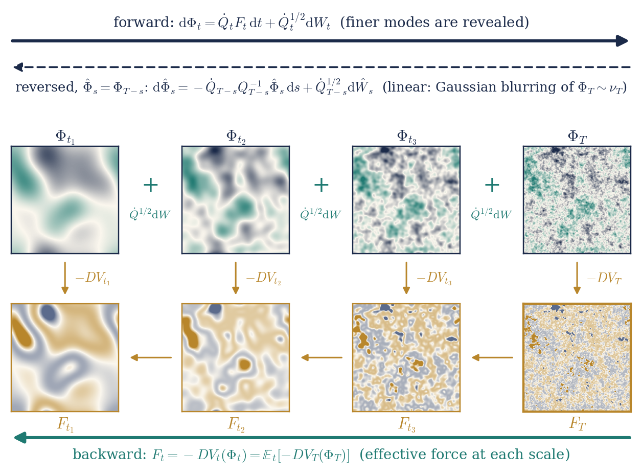
|
Figure 7.1. The forward–backward
structure of |
|
Abstract
Building on the scale decomposition and the stochastic observables of Lecture 3, we introduce interactions. The interacting measure can be generated in three ways: as a renormalisation group decomposition of the covariance, as an optimal control problem, whose dynamic programming equation is the Polchinski equation, and as a filtering problem: the field at resolution \(t\) is a noisy observation of the terminal field, the Polchinski process is this observation written in its own filtration, and backward in resolution its dynamics is linear, with Gaussian transitions, started from the interacting measure. The three views meet in one forward–backward system for a field and a force, and its natural coordinates are the force coordinates: the forward equation loses its drift, and the conditional covariance becomes the propagator. All this can be said in terms of forces, propagators and covariances. In the gradient case there is a parallel story for potentials: the value function generates the canonical transformation to force coordinates, the Legendre transform of the log-partition function of the filter gives the effective average action, and its flow is the Wetterich equation. Lecture 5 continues with the observables of the interacting theory, the Euclidean field equation and Nelson's Euclidean noise, the field equation at every resolution with its sub-Gaussian noise, and infinite volume, and contains the appendices. The treatment is formal: we compute as if all objects were smooth and integrable, and we indicate where the real difficulties lie.
The results presented in Lectures 4–7 were obtained recently, with the use of AI, in collaboration with Sarah-Jean Meyer.
Introduction 2
Structure 2
What is formal 2
Conventions 2
Acknowledgements 2
Main lecture 2
7Three ways to generate the interacting measure 2
7.1Renormalisation: decomposing the covariance 3
The field as a process 4
7.2Optimal control: the Polchinski equation 5
The control problem 6
Euler–Lagrange equation \(=\) FBSDE 6
Entropy 6
Generating functionals 6
Pontryagin's maximum principle 7
The costate is a gradient 7
The Hamiltonian of the field 7
With noise 8
7.3Filtering: measuring the field 8
The terminal field as a hidden signal 8
Generation by denoising 10
Literature: Polchinski, Eldan and diffusion models 11
7.4Where the three views meet 11
Exercises 12
8Force coordinates and potentials 13
8.1The force and a Burgers equation 13
8.2Removing the predictable drift 14
8.3The FBSDE in the forecast coordinate 14
A one-dimensional model: Burgers and Lax–Oleinik 15
8.4Conditional moments 16
Brascamp–Lieb and Cramér–Rao bounds 16
8.5Potentials: the value function as a generator 17
Phase space and Lagrangian graphs 17
The free action generates the shear 17
The value function generates the graph 18
No convexity is needed 18
8.6The Legendre transform and Wetterich's equation 19
Probabilistic meaning of \(\Gamma\) 21
8.7Variational meaning and the tree level 21
Constrained free energies 21
The tree level 22
Exercises 22
References 23
In Lecture 3 we decomposed the Gaussian free field along a resolution parameter and took as primary objects the stochastic observables: martingales in the filtration of finite-resolution measurements [BCG26]. In this lecture we introduce interactions, and we tell one story from three points of view: renormalisation, optimal control and filtering. See also [Pol84, BK87, Sal99, BBD24] for the renormalisation group side and [BG20, BG23] for the variational side.
Fix a finite volume \(\mathcal{M}=\mathbb{T}^d_L\) and a terminal resolution \(T < \infty\), which plays the role of an ultraviolet cutoff: the reference field \(X_T \sim \mu^{Q_T}\) is smooth. Let \(V_T\) be an interaction, a functional of smooth fields bounded below. Our main example is
| \(\displaystyle V_T (\varphi) = \int_{\mathbb{T}^d_L} \left[ \frac{\lambda}{12} H_4 (\varphi (x) ; c_T) + \gamma_T \hspace{0.17em} H_2 (\varphi (x) ; c_T) \right] \mathrm{d} x,\) | (7.1) |
with a mass counterterm \(\gamma_T\) to be fixed in Appendix A.2 of Lecture 5 (\(\gamma_T = 0\) for \(d = 2\)). The coupling is normalised by \(\lambda / 12\) so that the curvature of the quartic term is \(\lambda \varphi^2\), as in Lectures 6–7. The interacting measure at cutoff \(T\) is
| \(\displaystyle \nu_T (\mathrm{d} \varphi) = Z_T^{- 1} \mathrm{e}^{- V_T (\varphi)} \mu^{Q_T} (\mathrm{d} \varphi) .\) | (7.2) |
How does the Gaussian scale decomposition of Lecture 3 generate \(\nu_T\)? There are three answers.
Renormalisation (Section 7.1). Split the covariance into shells and integrate them out one at a time. At every resolution the field is again a Gibbs measure, and it is driven by an effective force.
Optimal control (Section 7.2). Steer the Gaussian field by a drift, at the least cost. The effective potential is the value function, and the Polchinski equation is the dynamic programming equation.
Filtering (Section 7.3). Observe the terminal field through noise, with increasing precision. The field at resolution \(t\) is the observation, the force is what it reveals about the terminal field, and backward in resolution the process has a linear dynamics with Gaussian transitions, started from the interacting measure.
Section 7.4 shows that the three constructions produce the same process. Throughout,
is the covariance still unresolved at resolution \(t\).
Decompose the covariance as in Lecture 3: \(Q_T = Q_t + S_t\), and correspondingly
with independent terms. Integrating out the second one defines the effective potential.
Definition
\(V_t\) is the interaction felt by the field at resolution \(t\) once the fluctuations between \(t\) and \(T\) have been integrated out: it is the Wilson effective action. At \(t = 0\), \(V_0 (0) = - \log Z_T\) is the free energy. Here is the first key fact.
Proposition
where \(\mathbb{P}_0\) is the law of the Gaussian process \(X\). Then \(\text{Law}_{\mathbb{P}} (X_T) = \nu_T\), and for every \(t \leqslant T\)
| \(\displaystyle \text{Law}_{\mathbb{P}} (X_t) = \nu_t, \qquad \nu_t (\mathrm{d} \varphi) := Z_T^{- 1} \mathrm{e}^{- V_t (\varphi)} \mu^{Q_t} (\mathrm{d} \varphi) .\) | (7.4) |
Moreover, the conditional law of \(X_T\) given \(\mathcal{F}_t\) is
Proof. Under \(\mathbb{P}_0\), \(X_T = X_t + (X_T - X_t)\) with an independent increment of law \(\mu^{Q_{T, t}}\). Hence \(\mathbb{E}_{\mathbb{P}} [G (X_t)] = Z_T^{- 1} \mathbb{E}_0 [G (X_t) \mathrm{e}^{- V_T (X_T)}] = Z_T^{- 1} \mathbb{E}_0 [G (X_t) \mathrm{e}^{- V_t (X_t)}]\). The conditional law follows in the same way.\(\Box\)
So at every resolution the field is again a Gibbs measure, with reference covariance \(Q_t\) and potential \(V_t\). The measure-valued martingale \((\mu_t^{X_t})_t\) goes from \(\nu_T\) at \(t = 0\) to \(\delta_{X_T}\) at \(t = T\): it is a stochastic localisation of \(\nu_T\) in the sense of Eldan [Eld23], adapted to the covariance profile [BBD24, BCG26].
Theorem
with \(\Phi_0 = 0\) and a \(\mathbb{P}\)-cylindrical Brownian motion \(W^{\mathbb{P}}\). In particular the effective force \((F_t)_{t \leqslant T}\) is a \(\mathbb{P}\)-martingale: an observable field of the interacting theory.
Proof. The density process is \(M_t := \mathbb{E}_0 [\hspace{0.17em} \mathrm{d} \mathbb{P}/ \hspace{0.17em} \mathrm{d} \mathbb{P}_0 |\mathcal{F}_t] = Z_T^{- 1} \mathrm{e}^{- V_t (X_t)}\), by Proposition 7.2. It is a martingale, so the drift in Itô's formula vanishes and \(\hspace{0.17em} \mathrm{d} M_t = - M_t \langle \mathrm{D} V_t (X_t), \dot{Q}_t^{1 / 2} \hspace{0.17em} \mathrm{d} W_t \rangle\). By Girsanov's theorem, \(W^{\mathbb{P}}_t = W_t + \int_0^t \dot{Q}_s^{1 / 2} \mathrm{D} V_s (X_s) \hspace{0.17em} \mathrm{d} s\) is a \(\mathbb{P}\)-Brownian motion, which is (7.6). Differentiating (7.3) gives \(\mathrm{D} V_t (\phi) = \mu_t^{\phi} (\mathrm{D} V_T)\), which is the second identity.\(\Box\)
Remark
is space-time harmonic for \(X\), \((\partial_t + L_t) h_t = 0\), and
this is the Polchinski equation
and the force is the logarithmic gradient of \(h\), \(F_t = \mathrm{D}
\log h_t (\Phi_t)\). Conditioning a Brownian motion on its endpoint is
the simplest example: \(h_t\) is then the Gaussian density of the
remaining increment, and the drift is that of the bridge
Read as an equation for an unknown pair \((\Phi, F)\),
Here and below we drop the superscript and write \(W\) for the Brownian
motion driving the interacting field. No equation for the potential is
needed to state
|
|
Figure 7.1. The forward–backward
structure of |
The measure \(\nu_T\) also solves a minimisation problem. Perturb the Gaussian field by an adapted drift, and pay for the drift and for the interaction at the endpoint. The effective potential is the value function of this problem. Its equation in \(t\), which we first derive directly from (7.3), is the dynamic programming equation.
Theorem
with terminal condition \(V_T\).
Proof. \(h_t = Z_T^{- 1} \mathrm{e}^{- V_t} = \mathrm{e}^{\frac{1}{2} \Delta_{Q_{T, t}}} h_T\) (Remark 7.4) is a Gaussian convolution, where \(\Delta_Q := \text{Tr} (Q \mathrm{D}^2)\). Since \(\partial_t Q_{T, t} = - \dot{Q}_t\), it solves the backward heat equation \(\partial_t h_t = - \frac{1}{2} \text{Tr} (\dot{Q}_t \mathrm{D}^2 h_t)\). Insert \(\mathrm{D}^2 h = (\mathrm{D} V \otimes \mathrm{D} V - \mathrm{D}^2 V) h\) and divide by \(- h\).\(\Box\)
The nonlinear term generates new, generally nonlocal, interactions (trees), and the trace term contracts pairs of fields with the covariance of the shell \([t, t + \mathrm{d} t]\) (loops). The substitution \(h \propto \mathrm{e}^{- V}\), which linearises the equation, is a Cole–Hopf transform: we come back to this in Section 8.1, and in Appendix A of Lecture 5.
the field driven by the control \(u\) under the Gaussian reference \(\mathbb{P}_0\).
The following result is standard in the stochastic optimal control setting, see e.g. Fleming and Soner's book [FS06]. A useful non-Markovian generalisation is given by Boué–Dupuis [BD98].
Theorem
| \(\displaystyle - \log \mathbb{E}_0 [\mathrm{e}^{- V_T (X_T)}] = V_0 (0) = \inf_{u \in \mathbb{H}_a} \mathbb{E}_0 \left[ V_T (X^u_T) + \frac{1}{2} \int_0^T \|u_s \|^2 \mathrm{d} s \right] .\) | (7.9) |
The infimum is attained at the feedback control \(u^{\ast}_s = -
\dot{Q}_s^{1 / 2} \mathrm{D} V_s (X^{u^{\ast}}_s)\), and \(\text{Law}
(X^{u^{\ast}}_T) = \nu_T\). The effective potential is the value
function, and
Proof. (Verification.) For any \(u\), by
Itô's formula and
with \(\mathrm{D} V_t = \mathrm{D} V_t (X^u_t)\) and a martingale \(M\). Integrating and taking expectations,
So the cost is \(\geqslant V_0 (0)\), with equality iff \(u =
u^{\ast}\). With this control \(X^{u^{\ast}}\) solves the same SDE as
\(\Phi\) in
| \(\displaystyle u_s = - \dot{Q}_s^{1 / 2} \hspace{0.17em} \mathbb{E}_s [\mathrm{D} V_T (X^u_T)] = \dot{Q}_s^{1 / 2} F_s .\) | (7.11) |
This is
Bounds on \(\mathcal{W}_T (f)\) uniform in \(T\), for \(f\) in a rich class, give tightness, moment bounds and the identification of limits. For \(\Phi^4_3\) the naive problem does not have uniform bounds: the leading-order optimal drift \(u_s \approx - \frac{\lambda}{3} \dot{Q}_s^{1 / 2} : X_s^3\): has a divergent cost. One renormalises by the change of variables \(u = - \frac{\lambda}{3} \dot{Q}^{1 / 2} : X^3 : + r\). After it, and after further paracontrolled changes of variables, the singular terms are explicit polynomials in the Wick powers of \(X\), cancelled by the counterterms, and the residual functional is coercive. Its control in Besov and paracontrolled norms, uniformly in \(T\), is the construction of \(\Phi^4_3\) in [BG20]; see also [BG21].
Pontryagin's principle [PBGM62] says that along an optimal pair \((x, u)\) there is a costate \(p\) such that
The state runs forward from its initial value, the costate backward from its terminal value: a two-point boundary value problem. In the smooth case the principle is the first-order condition. If \(\xi = \partial_{\varepsilon} x\) is the variation of the state under \(u \to u + \varepsilon v\), then \(\dot{\xi} = \partial_x b \xi + \partial_u bv\), \(\xi_t = 0\), and the costate equation is exactly what makes \(\frac{\mathrm{d}}{\mathrm{d} s} \langle p, \xi \rangle = \langle \partial_x \ell, \xi \rangle + \langle p, \partial_u bv \rangle\). Integrating over \([t, T]\) and using the terminal condition,
So the costate is the Lagrange multiplier of the constraint \(\dot{x} = b\), and an optimal control is a critical point of the Hamiltonian.
Its characteristics are Hamilton's equations for \(\mathcal{H}_{\ast}\), and along them \(p_s = - \mathrm{D} V (s, x_s)\): the costate is the sensitivity of the optimal cost to a displacement of the state, i.e. the force that the future exerts on the present.
is the Hamiltonian of a free particle with mass matrix \(\dot{Q}_s^{- 1}\): it does not depend on the state. Hence \(\dot{p} = 0\) and \(\dot{x} = \dot{Q}_s p\): the costate is conserved, and from \(t\) to \(T\) the state moves along the linear shear
| \(\displaystyle \Sigma_t : (x, p) \longmapsto (x + S_t p, \hspace{0.27em} p) . \) | (7.13) |
Its trajectories are the characteristics of the transport part of
The martingale term \(\Upsilon \mathrm{d} W\) is the price of
adaptedness: the costate may not anticipate the noise. For the field
\(\partial_x \mathcal{H}= 0\), so the costate is a martingale, \(p_t
=\mathbb{E}_t [- \mathrm{D} V_T (X_T)]\), and since the value function
is the effective potential (Theorem 7.6), \(p_t = -
\mathrm{D} V_t (X_t)\). The noise adds the Itô term to the
Hamilton–Jacobi equation, which becomes the Polchinski equation
In the notation of Theorem 7.6 the controlled field is
\(\mathrm{d} X = \dot{Q}_t^{1 / 2} (u \hspace{0.17em} \mathrm{d} t +
\mathrm{d}
W)\) and the optimal control is \(u_t = \dot{Q}_t^{1 / 2}
p_t\) (Exercise 7.3). Since \(p_t\) is the value \(F_t\) of
the force, the FBSDE
the field \(\Phi\) is the state, and the force \(F\) is the costate.
Stochastic localisation was introduced by Eldan [Eld13] to study measures in high dimension (see [Eld23] for a survey). The idea is to write a measure as a mixture of simpler ones, through a measure-valued martingale driven by noise. Proposition 7.2 says that the Polchinski process does exactly this for \(\nu_T\). What Eldan's construction adds to the picture of Section 7.1 is a statistical reading:
the Polchinski process is a noisy observation of its own terminal value, and its drift is what an optimal filter learns from this observation.
| \(\displaystyle \Phi_t = J_t \Phi_T + \zeta_t, \quad \zeta_t \sim N (0, Q_t (1 - J_t)), \quad \text{independent of } \Phi_T . \) | (7.14) |
Read
| \(\displaystyle \mathrm{d} \Phi_t = \dot{Q}_t S_t^{- 1} (\Phi_T - \Phi_t) \hspace{0.17em} \mathrm{d} t + \dot{Q}_t^{1 / 2} \hspace{0.17em} \mathrm{d} B_t,\) | (7.15) |
with \(B\) a Brownian motion independent of \(\Phi_T\), in the filtration enlarged by \(\sigma (\Phi_T)\): at each resolution the field is pulled towards the hidden terminal field, and the pull is seen through noise. The filtering problem is to estimate \(\Phi_T\) from \(\mathcal{F}_t = \sigma (\Phi_s : s \leqslant t)\), the filtration of the Polchinski process itself. Let \(\psi_t =\mathbb{E}_t [\Phi_T]\), \(\text{Cov}_t = \text{Cov} (\Phi_T |\mathcal{F}_t)\), and let
be the regulator.
Proposition
The conditional law of \(\Phi_T\) given \(\mathcal{F}_t\) is the Bayesian posterior
| \(\displaystyle \mu_t^{\Phi_t} (\mathrm{d} y) \propto \mathrm{e}^{\langle S_t^{- 1} \Phi_t, y \rangle - \frac{1}{2} \langle y, \mathcal{R}_t y \rangle} \nu_T (\mathrm{d} y) .\) | (7.16) |
It depends on the path only through \(\Phi_t\), a sufficient statistic, and \(\mathcal{R}_t\) is the precision gained on \(\Phi_T\).
The Brownian motion \(W\) of the FBSDE
and the force is the posterior mean of the pull in
So
Every observable \(O_t =\mathbb{E}_t [G (\Phi_T)]\) solves the filter equation
in particular
Proof. (a) By Proposition 7.2 the
conditional law is \(\mu_t^{\Phi_t}\), the tilt of \(\mu^{S_t} (\cdot -
\Phi_t)\) by \(\mathrm{e}^{- V_T}\). The ratio of the Gaussian densities
of \(\mu^{S_t} (\cdot - x)\) and \(\mu^{Q_T}\) at \(y\) is
\(\mathrm{e}^{\langle S_t^{- 1} x, y \rangle - \frac{1}{2} \langle
y,
\mathcal{R}_t y \rangle}\) up to a function of \(x\); equivalently,
apply Bayes' formula to the likelihood of
So the Polchinski process is a filter. The interacting measure is the prior on a hidden field; at resolution \(t\) one has observed the coarse field \(\Phi_t\), and \(\mu_t^{\Phi_t}\) is what is known about the fine one. The forecast \(\psi_t\) is the posterior mean of the hidden field, and \(\dot{Q}_t F_t\) is the posterior mean of its pull on the observed one. For the Gaussian prior \(\mu^{Q_T}\) the increments are independent, so the posterior mean is \(\Phi_t\) itself and \(F = 0\): \(\Phi_t\) is the estimate that ignores the interaction and \(\psi_t\) the one that includes it. The effective potential is a likelihood ratio: by the proof of Theorem 7.3, \(Z_T^{- 1} \mathrm{e}^{- V_t (\Phi_t)}\) is the likelihood ratio of the observation up to resolution \(t\) under the interacting and under the Gaussian prior, and the Polchinski equation is the equation of its logarithm.
Proposition
with \(\hat{W}\) a Brownian motion independent of \(\Phi_T\), and
its solution is
Proof. Under \(\mathbb{P}_0\), \(X\) is a
centred Gaussian process with independent increments, so its reversal is
a Gaussian Markov process: for \(t < u\), the law of \(X_t\) given
\((X_r)_{r \geqslant u}\) is \(N (Q_t Q_u^{- 1} X_u, Q_t - Q_t Q_u^{- 1}
Q_t)\), and letting \(u \downarrow t\) gives the drift and the diffusion
of
the force is the score of \(\nu_t\) relative to that of the Gaussian reference \(\mu^{Q_t}\), as \(\nu_t \propto \mathrm{e}^{- V_t} \mu^{Q_t}\) requires. The forecast is the optimal denoiser, and Tweedie's formula
is again \(\psi_t = \Phi_t + S_t F_t\). This is the structure of score-based generative models (diffusion models), with \(\nu_T\) as the data distribution, the blurring as the noising process and the Polchinski process as the generating dynamics.
Remark
\(\dot{Q}_t\) times the score of the density \(p_t\) of the field at that scale. Reversing the direction of resolution compensates the drift exactly up to the score. For the free field \(b_t = 0\) and \(\mathrm{D} \log p_t (x) = - Q_t^{- 1} x\), so the whole backward drift is the Gaussian score; with an interaction, the score carries everything that the backward dynamics ignores. In Nelson's stochastic mechanics [Nel67] \(b_{\ast}\) is the backward velocity, and the half difference \(\frac{1}{2} (b - b_{\ast}) = \frac{1}{2} \dot{Q}_t \mathrm{D} \log p_t\) is the osmotic velocity. The same score is the noise of the field equation of Lecture 5, the observable \(\omega_t = K \Phi_t - J_t F_t\) of Section 9.3 there: by (9.14) of Lecture 5,
so the noise at resolution \(t\) is, up to the smoothing \(J_t\), the part of the drift that time reversal does not compensate.
Remark
| \(\displaystyle j_t =\mathcal{R}_t \Phi_T + N_t, \quad N_t = S_t^{- 1} \zeta_t, \quad \mathbb{E} [N_s \otimes N_t] =\mathcal{R}_{s \wedge t}, \quad N \text{ independent of } \Phi_T . \) | (7.18) |
In this coordinate
and
up to a function of \(t\). Then \(\psi_t = \mathrm{D} \mathcal{K}_t (j_t)\), \(\text{Cov}_t = \mathrm{D}^2 \mathcal{K}_t (j_t)\), \(\hspace{0.17em} \mathrm{d} j_t = \dot{\mathcal{R}}_t \psi_t \hspace{0.17em} \mathrm{d} t + \dot{\mathcal{R}}_t^{1 / 2} \hspace{0.17em} \mathrm{d} W_t\) with the same innovation \(W\), and
the Polchinski equation in the variable \(j\) [BBD24] (\(\partial_t \mathcal{K}= - \frac{1}{2} \mathbb{E} \langle y, \dot{\mathcal{R}} y \rangle\) and \(\text{Tr} (\dot{\mathcal{R}} \mathrm{D}^2 \mathcal{K}) =\mathbb{E} \langle y, \dot{\mathcal{R}} y \rangle - \langle \psi, \dot{\mathcal{R}} \psi \rangle\), expectations under the posterior). The basic form of Eldan's scheme is the profile \(S_t = (Q_T^{- 1} + t)^{- 1}\), \(t \in [0, \infty)\) (the terminal resolution is then \(t = \infty\), and \(Q_T\) is the cutoff covariance), where \(\mathcal{R}_t = t\) and \(j_t = t \Phi_T + N_t\) with \(N\) a Brownian motion; Eldan's original construction [Eld13] uses an adapted control matrix. After the change of variable \(q = q_0 + t^2\), and with \(Q_T\) replaced by the full covariance \(C\), this is the mass-regulator profile of Exercise 8.8, used in Lectures 6–7.
The three constructions give one process. Renormalisation produces it as the field at resolution \(t\) with its effective drift (Theorem 7.3), control as the optimal state (7.11), and filtering as the observation written in its own filtration (Proposition 7.7). Each of them has a name for each object:
|
Renormalisation |
Control |
Filtering |
\(t\) |
resolved covariance \(Q_t\) |
time of the problem |
information gained \(\mathcal{R}_t\) |
\(\Phi_t\) |
field at resolution \(t\) |
state |
observation; posterior mean for the Gaussian prior |
\(F_t\) |
effective force |
costate |
posterior mean of the terminal force |
\(W\) |
fresh fluctuation of the shell |
noise of the controlled field |
innovation |
\(S_t\) |
unresolved covariance |
free motion from \(t\) to \(T\) |
posterior covariance for the Gaussian prior |
\(\psi_t = \Phi_t + S_t F_t\) |
mean of the conditional law \(\mu_t^{\Phi_t}\) |
terminal state predicted by free motion |
posterior mean |
\(\text{Cov}_t\) |
covariance of \(\mu_t^{\Phi_t}\) |
\(S_t - S_t \mathrm{D}^2 V_t S_t\) |
posterior covariance |
\(V_t\) |
effective potential |
value function |
minus the log-likelihood ratio of the observation, up to \(\log Z_T\) |
In the last column, \(\Phi_t\) is the estimate of the terminal field that ignores the interaction, and \(\psi_t\) is the estimate that includes it. Their difference is \(S_t F_t\): the force is what the interaction adds to the estimate, in units of the free propagator \(S_t\). The conditional covariance \(\text{Cov}_t\) replaces \(S_t\) as the propagator. Forces, propagators and covariances are the common language of the three views, and the next section writes the system in it. Only the last row of the table, and the formula for \(\text{Cov}_t\) in the control column, involve a potential.
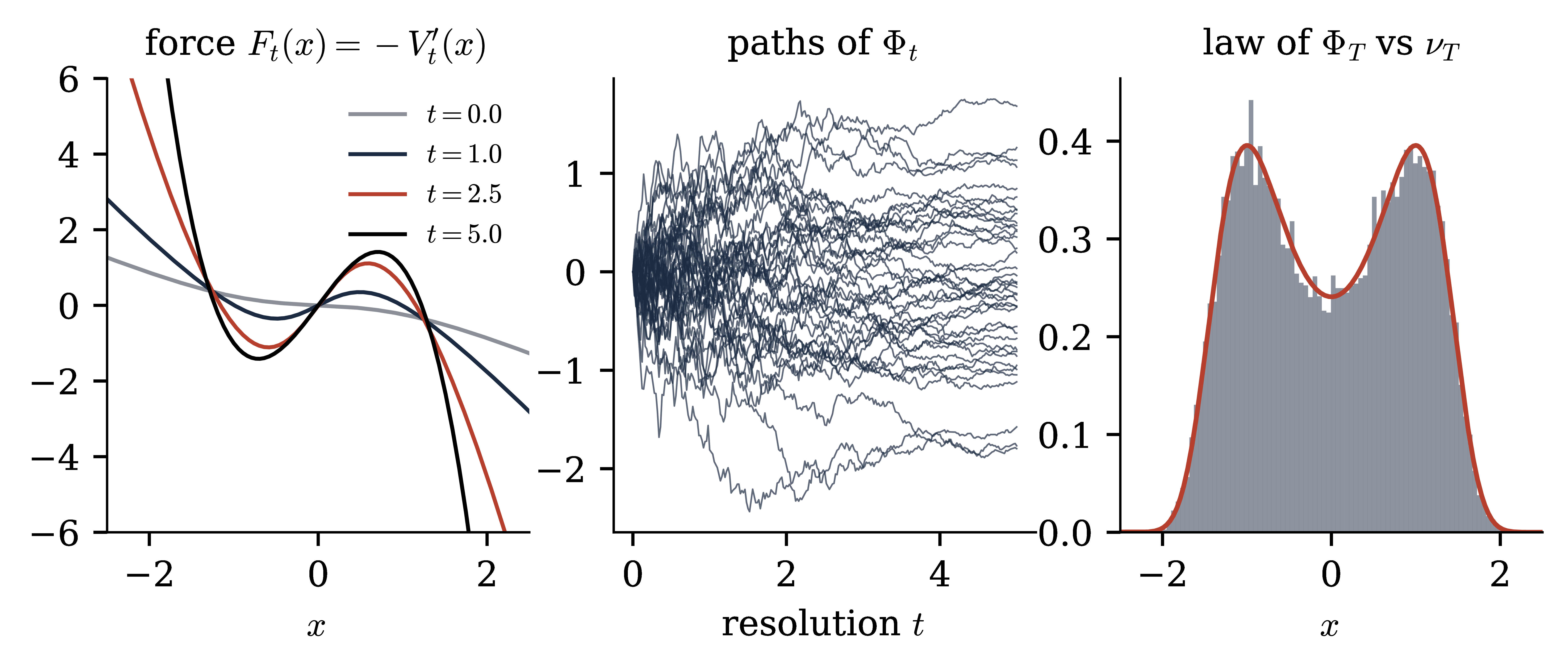
|
Figure 7.2. A zero-dimensional Polchinski
process (Exercise 7.2): \(Q_t = 1 - \mathrm{e}^{-
t}\), \(T = 5\), \(V_T (x) = \frac{1}{2} x^4 - \frac{3}{2}
x^2\). Left: the effective force \(F_t = - V_t'\) is almost
linear at low resolution and develops the double-well structure
as \(t \to T\). Centre: paths of the FBSDE |
Exercise
Exercise
Exercise
Exercise
Exercise
The three views agree on the forward–backward system (7.7), which from now on is the primary object, with a martingale force \(F_t = F_t (\Phi_t)\), \(\hspace{0.17em} \mathrm{d} F_t = \Upsilon_t \hspace{0.17em} \mathrm{d} W_t\). We look for the coordinates in which it is simplest. They are suggested by the table above: the posterior mean \(\psi\), which we call the forecast, and the force. They remove the predictable part of the forward dynamics, and they integrate exactly the bilinear (tree) part of the force flow.
Sections 8.1–8.4 tell this story in terms of forces, propagators and covariances. The potential enters only through the terminal force and, for a gradient force, through the identification of the response with the conditional covariance; the system in force coordinates makes sense for a force that is not a gradient. Sections 8.5–8.7 tell it again in terms of potentials: the value function generates the canonical transformation to force coordinates, the Legendre transform connects it to the filter, and the equation for the force is the Wetterich equation for the effective average action [Wet93, BTW02].
Differentiating
| \(\displaystyle \partial_t F_t = - \mathrm{D} F_t [\dot{Q}_t F_t] - \tfrac{1}{2} \text{Tr} (\dot{Q}_t \mathrm{D}^2 F_t), \qquad F_T = - \mathrm{D} V_T,\) | (8.1) |
an infinite-dimensional, backward, viscous Burgers equation.
The Cole–Hopf transform \(F = \mathrm{D} \log h\) linearises it,
which is the statement that \(h \propto \mathrm{e}^{- V}\) solves a heat
equation. Two remarks on
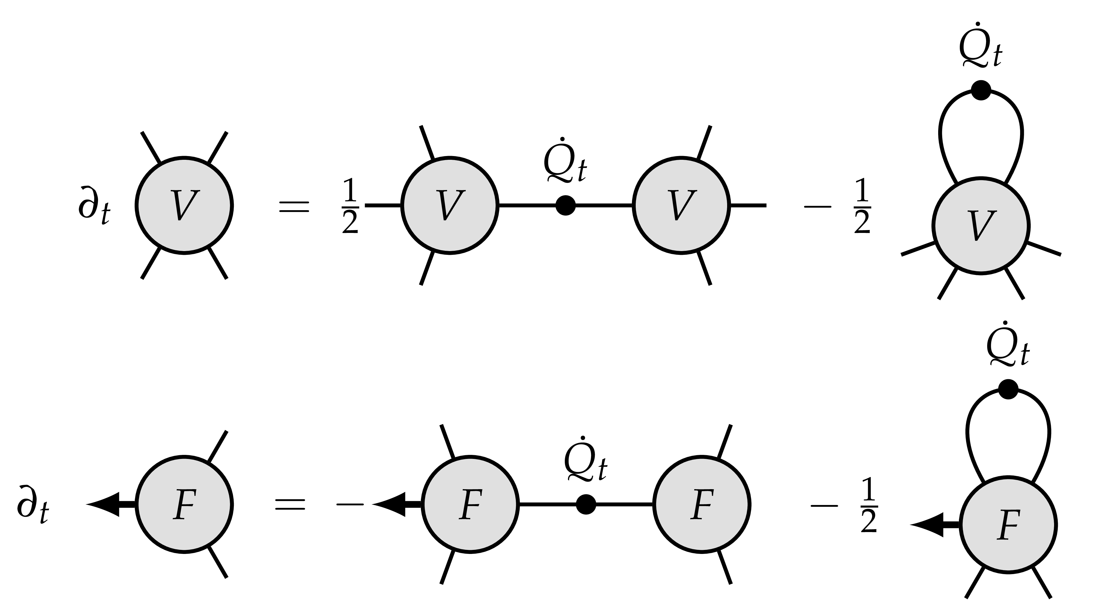
|
Figure 8.1. The Polchinski equation
|
it uses only the force, which is a local quantity (intensive), while \(V_t\) is extensive, of order of the volume. This matters in infinite volume (Section 9.5 of Lecture 5);
the Burgers flows for different covariances commute when \(\mathrm{D} F_t\) is symmetric, i.e. when \(F_t\) is a gradient [BCG26]: then \(F_t = - \mathrm{D} V_t\), the flows are gradients of Polchinski flows, i.e. of Gaussian convolutions after the Cole–Hopf transform, and Gaussian convolutions commute. For a non-gradient force, as for the general Wilson–Itô diffusions of [BCG26], the flows do not commute.
The function \(F_t (\cdot)\) with \(F_t = F_t (\Phi_t)\) is the
decoupling field of the FBSDE, and the Burgers equation
The drift \(\dot{Q}_t F_t\) of the state is predictable, and the costate
is a martingale. Hence the drift that remains to be accumulated on \([t,
T]\) is predicted, at resolution \(t\), by transporting the current
state with the current costate along the free flow
Proposition
| \(\displaystyle \psi_t := \mathbb{E}_t [\Phi_T] = \Phi_t + S_t F_t,\) | (8.2) |
i.e. \((\psi_t, F_t) = \Sigma_t (\Phi_t, F_t)\). It is a martingale, with
Proof. The identity is in the proof of Proposition 7.7(b), and uses no commutativity. For the differential, the drift \(\dot{Q}_t F_t\) of \(\Phi\) cancels against \(\dot{S}_t F_t\), and \(S_t \hspace{0.17em} \mathrm{d} F_t = S_t \Upsilon_t \hspace{0.17em} \mathrm{d} W_t\).\(\Box\)
So \(\psi\) is a closed observable, the field observable of [BCG26]. The field splits as
| \(\displaystyle \Phi_t = \psi_t - S_t F_t :\) | (8.4) |
a martingale, minus the drift still expected on the unresolved scales,
which vanishes at \(t = T\). The noise of \(\psi\) in
Assume that the map
is invertible, and write its inverse as
| \(\displaystyle x = \psi + S_t \mathcal{F}_t (\psi), \qquad \mathcal{F}_t (\psi) := - F_t (x),\) | (8.5) |
so that \(F_t = -\mathcal{F}_t (\psi_t)\): the costate is now a function of the forecast. Introduce the response, and recall the regulator of the filter:
Differentiating the two maps \(x \leftrightarrow \psi\) gives
Theorem
with \(\psi_0 = S_0 F_0 =\mathbb{E} [\Phi_T]\) and \(\psi_T = \Phi_T\). The forward equation has no drift, and its covariance is
The decoupling field \(\mathcal{F}\) solves the pure diffusion equation
Proof. The forward equation is
The backward equation is \(F_t =\mathbb{E}_t [F_T]\) with \(\psi_T =
\Phi_T\). Since \(\mathcal{F}_t (\psi_t)\) is a martingale and \(\psi\)
has no drift, the drift in Itô's formula for \(\mathcal{F}_t
(\psi_t)\) is the left-hand side of
Compare
Along the characteristics \(x = y + sg' (y)\) the velocity is constant, \(u (s, y + sg' (y)) = g' (y)\): in the Lagrangian label \(y\) the transport term disappears, and nothing moves. As long as the characteristics do not cross, i.e. \(1 + sg'' > 0\), the map \(y \mapsto x\) is invertible, and \(u = \partial_x G\) with the potential given by the Lax–Oleinik formula (or Hopf–Lax formula)
whose minimiser \(y (s, x)\) is the Lagrangian label of the point \(x\). After the characteristics cross, the formula still selects one label, the entropy solution, and \(u\) has shocks. The viscous equation \(\partial_s u + u \partial_x u = \varepsilon \partial_x^2 u\) is linearised by the Cole–Hopf transform,
and \(G^{\varepsilon} \to G\) as \(\varepsilon \to 0\) by Laplace's method.
The dictionary with this section is: the unresolved covariance \(S_t\)
is the time \(s\), the field \(x\) is the Eulerian point, the forecast
\(\psi\) is the Lagrangian label \(y\), \(- F_t = \mathrm{D} V_t\) is
the velocity \(u\) (and \(V_t\) is \(G\)), and \(V_T\) is the datum
\(g\). The shear
Theorem 8.2 is the Lagrangian description of the
viscous problem. With noise the label is no longer a function
of the Eulerian point: it is its posterior mean, the mean \(\psi\) of
\(y\) under the Cole–Hopf measure \(\propto \mathrm{e}^{- g (y) -
(x - y)^2 / 2 s}\), which is \(\mu_t^x\). In this label the velocity is
no longer constant but a martingale, and its evolution
For the Polchinski process the response has a direct meaning.
Proposition
In particular \(H_t > 0\) is symmetric, \(\mathbb{1} + S_t \mathrm{D} F_t = \text{Cov}_t S_t^{- 1}\) is always invertible, and \(H_t \leqslant S_t\) when \(V_T\) is convex.
Proof. By
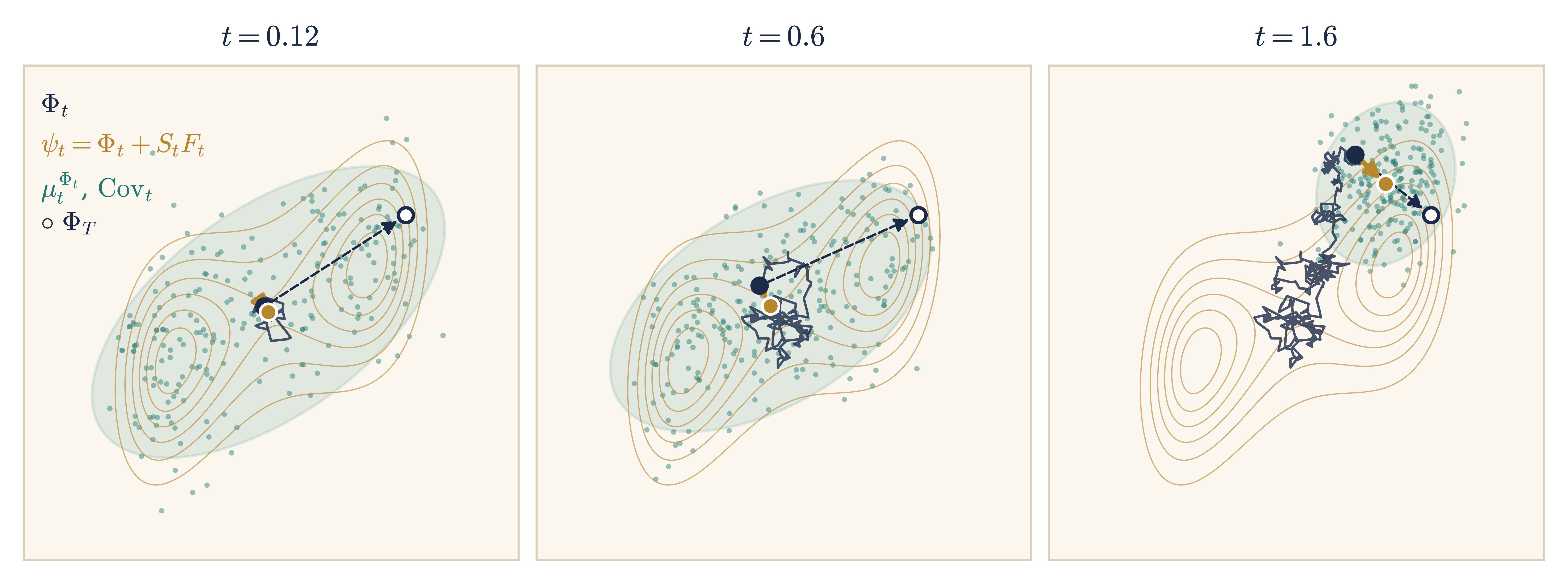
So the forecast and the response are the first two conditional moments of the stochastic localisation \(\mu_t^{\Phi_t}\) of Proposition 7.2: \((\psi_t, \text{Cov}_t) = (\mathbb{E}[\Phi_T \hspace{0.17em} | \hspace{0.17em} \Phi_t], \text{Cov} (\Phi_T \hspace{0.17em} | \hspace{0.17em} \Phi_t))\) (Figure 8.2). They are tied by Itô's formula: since \(\mathbb{E}_t [\Phi_T \otimes \Phi_T] = \psi_t \otimes \psi_t + \text{Cov}_t\) is a martingale,
Conditional variance is resolved at the rate \(\text{Cov}_t \dot{\mathcal{R}}_t \text{Cov}_t\), which for the Gaussian reference is \(S_t \dot{\mathcal{R}}_t S_t = \dot{Q}_t\).
The lower bound follows from \(\mathbb{E}_{\mu} [(y - m) \otimes \mathrm{D} \mathcal{U}(y)] = 1\) (integration by parts) and the Cauchy–Schwarz inequality, with the Fisher information \(\mathbb{E}_{\mu} [\mathrm{D} \mathcal{U} \otimes \mathrm{D} \mathcal{U}] =\mathbb{E}_{\mu} \mathrm{D}^2 \mathcal{U}\) (Exercise 8.9). The two bounds coincide when \(V_T\) is quadratic, and their gap is a Jensen gap for the inverse. Through Proposition 8.3 they are two-sided bounds on the Hessian of the effective potential, i.e. on the response \(H_t\), which is the propagator of the Wetterich equation below. Some consequences:
If \(V_T\) is convex, then \(\operatorname{Cov}_t \leqslant S_t\): the interaction can only reduce the conditional variance. Equivalently \(\mathrm{D}^2 V_t \geqslant 0\): convexity is preserved along the Polchinski flow (as also follows from the Prékopa–Leindler inequality).
If \(\mathrm{D}^2 V_T \geqslant \kappa\) with \(\kappa > 0\), then \(\operatorname{Cov}_t \leqslant (S_t^{- 1} + \kappa)^{- 1}\) uniformly in the conditioning: a uniform mass in the interaction is a uniform mass in every conditional law.
For \(\Phi^4_3\) convexity is already lost through the Wick
ordering: \(H_4 (\varphi ; c_T) = \varphi^4 - 6 c_T \varphi^2 + 3
c_T^2\), so
|
Figure 8.2. Stochastic localisation for a
two-component field: \(Q_t = (1 - \mathrm{e}^{- t})
\mathbb{1}\), \(T = 4\), \(V_T\) a tilted double well, and the
contours show the density of \(\nu_T\). One path of |
We now use that the force is a gradient, \(F_t = - \mathrm{D} V_t\), whose graph is a Lagrangian submanifold, and that \(V_t\) is the value function of Theorem 7.6. In Hamilton–Jacobi theory a value function is more than a cost: it generates a canonical transformation. A complete family of solutions of the Hamilton–Jacobi equation generates the transformation that trivialises the dynamics. Force coordinates are this transformation.
| \(\displaystyle \mathcal{A}_t (x, \psi) = \frac{1}{2} \langle \psi - x, S_t^{- 1} (\psi - x) \rangle . \) | (8.10) |
The relation \(\psi = x + S_t p\) is the shear (7.13). Since \(\mathrm{D}_x \mathcal{A}_t = - p\) and \(\mathrm{D}_{\psi} \mathcal{A}_t = p\), at fixed \(t\)
so \(\mathcal{A}_t\) is the generating function of the canonical transformation \(\Sigma_t\). Moreover
for every \(\psi\) it solves the noiseless Polchinski equation, so it is a complete integral of that equation, with parameter \(\psi\). Jacobi's theorem then says that in the new coordinates the Hamiltonian \(\mathcal{H}_{\ast}\) vanishes: \(\psi\) and \(p\) are constants of motion.
This is what force coordinates are:
\((\psi_t, F_t)\) are the Jacobi coordinates of the free Hamiltonian of the field.
The noise does not destroy this: the constants of motion become martingales, \(\psi_t\) by Proposition 8.1 and \(F_t\) by Theorem 7.3. The only dynamics left is their quadratic variation.
| \(\displaystyle \mathcal{F}_t = \mathrm{D} \Gamma_t, \qquad H_t = (S_t^{- 1} + \mathrm{D}^2 \Gamma_t)^{- 1}, \qquad \Gamma_T = V_T .\) | (8.11) |
These two generating functions are related by the Moreau (infimal convolution) transform
| \(\displaystyle V_t (x) = \inf_{\psi} \left\{ \Gamma_t (\psi) + \tfrac{1}{2} \langle x - \psi, S_t^{- 1} (x - \psi) \rangle \right\},\) | (8.12) |
whose optimality conditions \(x = \psi + S_t \mathrm{D} \Gamma_t
(\psi)\), \(\mathrm{D} V_t (x) = \mathrm{D} \Gamma_t (\psi)\) are
At the minimiser, \(V_t (x) = \Gamma_t (\psi) +\mathcal{A}_t (x, \psi)\): the value function is the cost \(\Gamma_t\) attached to the forecast, plus the cost of reaching the forecast by free motion. This is the rule for transporting a generating function along a canonical transformation:
since \(\mathrm{D} \Gamma_t (\psi) = - F_t = - p\).
For \(\Gamma_t\) one only gets semiconvexity, \(S_t^{- 1} + \mathrm{D}^2
\Gamma_t =\operatorname{Cov}_t^{- 1} > 0\), i.e. \(\Gamma_t +
\frac{1}{2} \langle \cdot, S_t^{- 1} \cdot \rangle\) is strictly convex,
which is what
|
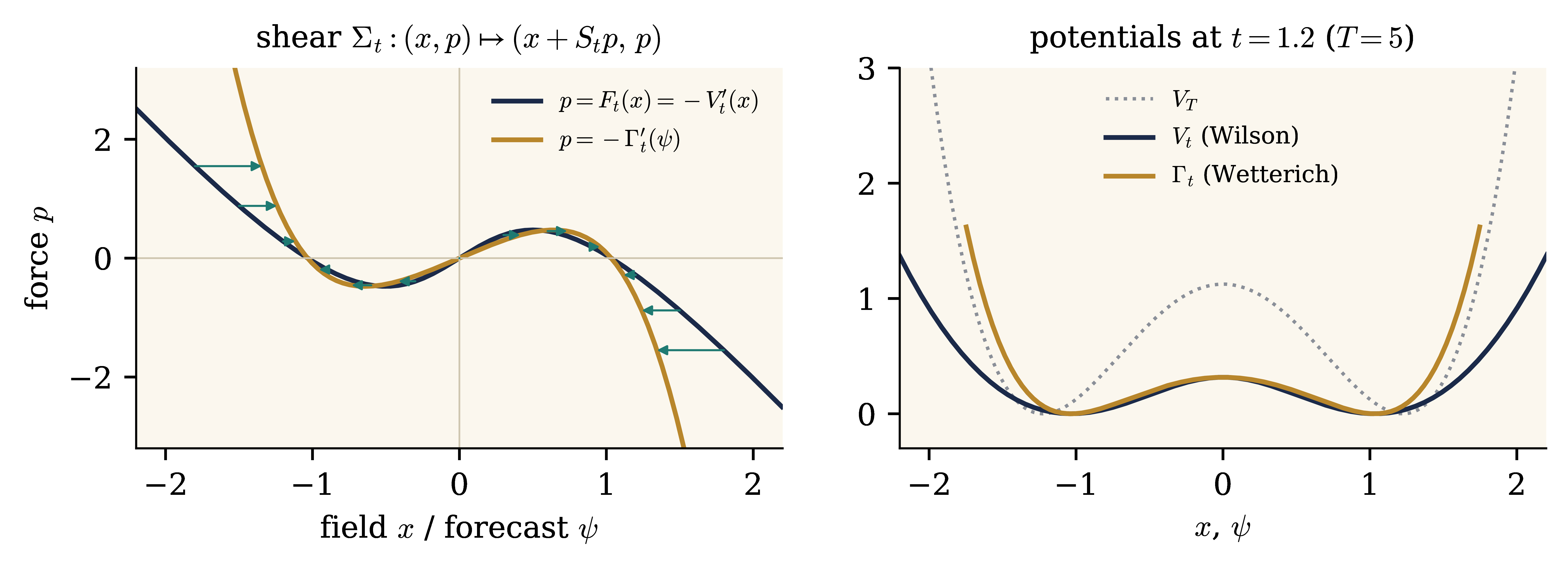
Figure 8.3. The zero-dimensional model of Figure 7.2 at \(t = 1.2\). Left: the shear \(\Sigma_t\) (teal arrows) maps the graph of the force \(F_t = - V_t'\) (navy) to a graph over the forecast \(\psi\) (gold), which is the graph of \(- \Gamma_t'\). Right: the bare potential \(V_T\), the effective potential \(V_t\) and \(\Gamma_t\), each shifted to have minimum \(0\). |
Theorem
| \(\displaystyle \partial_t \Gamma_t = \tfrac{1}{2} \text{Tr} [\dot{\mathcal{R}}_t ((S_t^{- 1} + \mathrm{D}^2 \Gamma_t)^{- 1} - S_t)], \qquad \Gamma_T = V_T .\) | (8.13) |
Equivalently, the effective average action \(\Gamma^{\text{EAA}}_t (\psi) := \Gamma_t (\psi) + \frac{1}{2} \langle \psi, Q_T^{- 1} \psi \rangle\) solves, up to a field-independent term,
| \(\displaystyle \partial_t \Gamma^{\text{EAA}}_t = \tfrac{1}{2} \text{Tr} [\dot{\mathcal{R}}_t (\mathrm{D}^2 \Gamma^{\text{EAA}}_t +\mathcal{R}_t)^{- 1}] .\) | (8.14) |
It interpolates between the bare action
(\(\mathcal{R}_T = \infty\)) and the 1PI effective action \(\Gamma^{\text{EAA}}_0\) of \(\nu_T\) (\(\mathcal{R}_0 = 0\)).
Proof. Integrate
Hence
Near \(t = T\) the two traces \(\text{Tr} (\dot{\mathcal{R}}_t (S_t^{-
1} + \mathrm{D}^2 \Gamma_t)^{- 1})\) and \(\text{Tr}
(\dot{\mathcal{R}}_t S_t) = \text{Tr} (S_t^{- 1} \dot{Q}_t)\) in
|
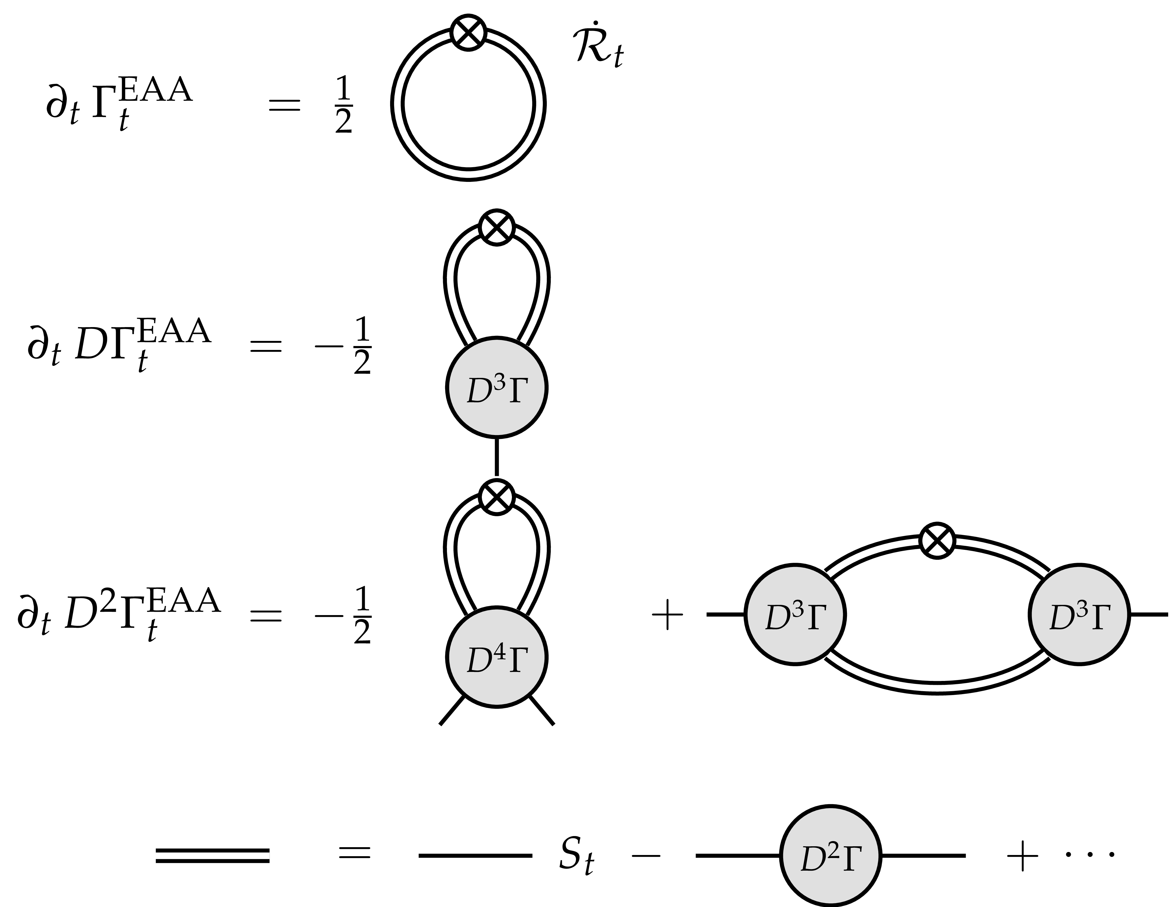
Figure 8.4. The Wetterich equation
|
Thus the Wetterich equation is the gradient-integrated form of the force
equation
Wetterich
FBSDE
field argument \(\psi\)
forecast \(\psi_t =\mathbb{E}_t [\Phi_T]\), the state
transported by \(\Sigma_t\)
\(\mathrm{D} \Gamma_t (\psi_t)\)
minus the costate, \(- F_t =\mathbb{E}_t [\mathrm{D}
V_T (\Phi_T)]\)
propagator \((\mathrm{D}^2 \Gamma^{\text{EAA}}_t
+\mathcal{R}_t)^{- 1}\)
conditional covariance \(\text{Cov}_t\)
regulator \(\mathcal{R}_t = S_t^{- 1} - Q_T^{-
1}\)
precision of the unresolved shell, minus that of the
prior
\(\partial_t \Gamma_t\)
\(\frac{1}{2} \text{Tr} [\dot{\mathcal{R}}_t
(\text{Cov}_t - S_t)]\)
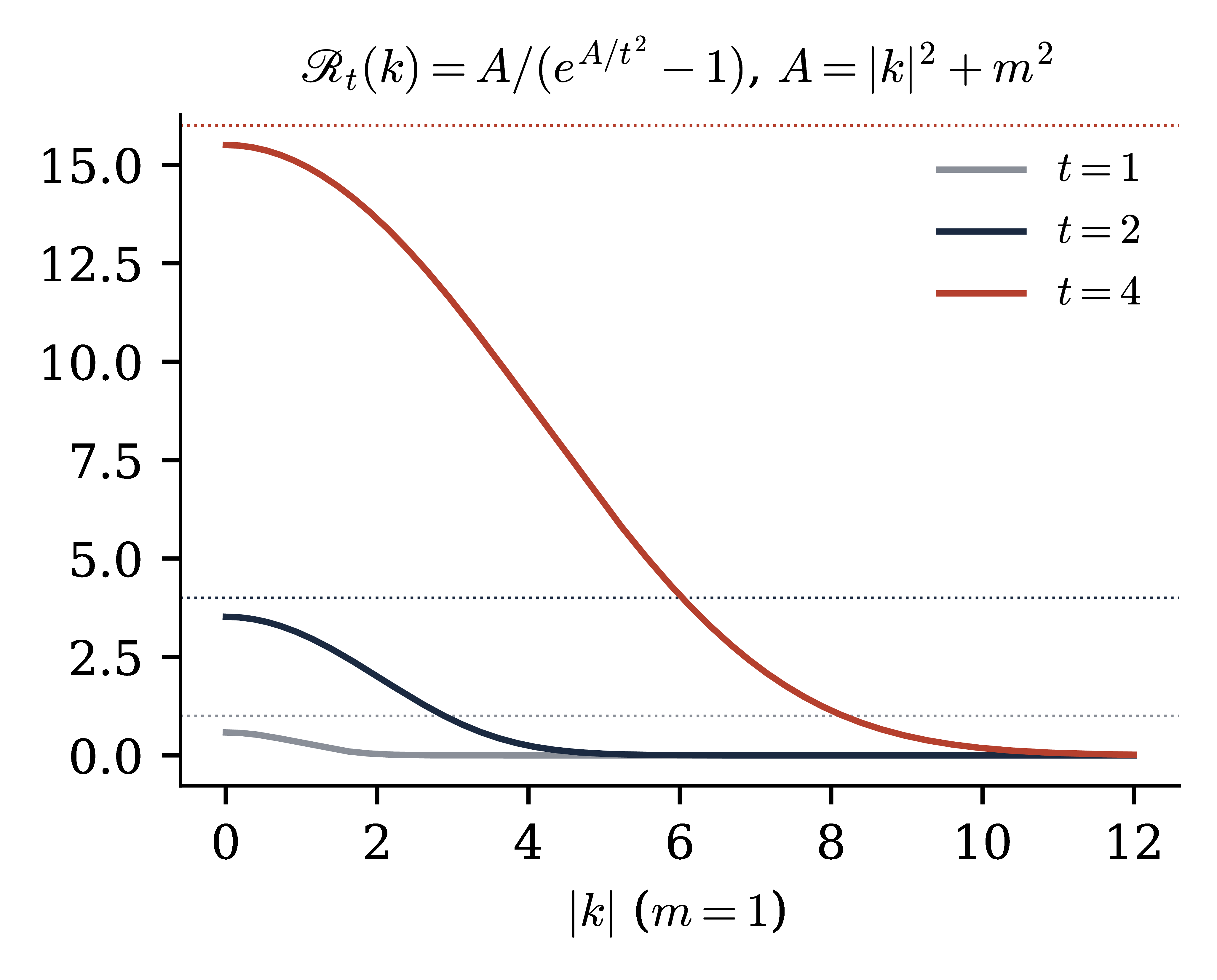
The flow of \(\Gamma\) is driven by the difference between the interacting and the free conditional covariances, paired with the shell \(\dot{\mathcal{R}}_t\). It is one-loop exact, with the full propagator inside the trace. In the Gaussian case \(\mathrm{D}^2 \Gamma_t\) is constant and only the constant term of \(\Gamma\) flows. For the heat profile with \(T = \infty\), \(S_t = C (1 - \mathrm{e}^{- A / t^2})\) and
| \(\displaystyle \mathcal{R}_t = \frac{A}{\mathrm{e}^{A / t^2} - 1},\) | (8.15) |
which behaves like a mass term \(t^2\) on the modes \(|k| \ll t\) (for \(m \ll t\)) and is exponentially small on the modes \(|k| \gg t\): the exponential regulator of the functional renormalisation group (Figure 8.5).
Proposition
up to a function of \(t\), and differentiating at fixed \(\psi\) gives the Wetterich equation (8.13) again.
Proof. By (8.12) and the formula
for \(\mathcal{K}\). At fixed \(\psi\), with \(j = \mathrm{D}
\mathcal{K}^{\ast} (\psi)\), the envelope theorem and
and \(\partial_t \frac{1}{2} \langle \psi, S^{- 1} \psi \rangle = \frac{1}{2} \langle \psi, \dot{\mathcal{R}} \psi \rangle\). Hence \(\partial_t \Gamma_t = \frac{1}{2} \text{Tr} (\dot{\mathcal{R}} \text{Cov})\) up to a function of \(t\), which is \(- \frac{1}{2} \text{Tr} (\dot{\mathcal{R}} S)\) with the normalisation (8.12).\(\Box\)
So one Lagrangian graph has three generators: \(V_t\) in the field \(x\), \(\mathcal{K}_t\) in the coordinate \(j = S_t^{- 1} x\) of Remark 7.10, and \(\Gamma_t\) in the forecast \(\psi\). The Polchinski flow is the Hamilton–Jacobi equation of the log-partition function of the localisation; the Wetterich flow is its Legendre dual [Mor94], whose argument is the posterior mean, and whose regulator is the information gained. At \(t = 0\), where \(\mathcal{R}_0 = 0\), \(\mathcal{K}_0\) is the generating function \(\Lambda\) of the cumulants of \(\nu_T\) below.
the generating functional of the vertex functions introduced by Jona-Lasinio [JL64]. It is a probabilistic object, as Jona-Lasinio emphasised in his probabilistic reading of the renormalisation group [JL75, JL01]; for the link with large deviations see Section VIII of [JL01]. By Cramér's theorem the empirical mean of \(N\) independent samples of \(\nu_T\) takes the value \(\psi\) with probability
so \(\Gamma^{\text{EAA}}_0 - V_0 (0)\) is the rate function of the large deviations of averages of the field. In particular \(\Gamma^{\text{EAA}}_0\) is convex even when \(V_T\) is not, it is minimal at the mean of \(\nu_T\), and its Hessian there is the inverse covariance. Formally the same holds for the field averaged over a large volume, with the volume as the large parameter and the effective potential of quantum field theory (\(\Gamma\) per unit volume at constant \(\psi\), not \(V_t\)) as rate function; in that limit flat parts may appear (the Maxwell construction).
for \(\nu\) of mean \(\psi\),
So \(\Gamma_t\), the effective average action up to the quadratic term
\(\frac{1}{2} \langle \psi, Q_T^{- 1} \psi \rangle\), is the free
energy of the unresolved shell constrained to the forecast \(\psi\), and
| \(\displaystyle V^{\text{tree}}_t (x) = \inf_y \left\{ V_T (y) + \tfrac{1}{2} \langle y - x, S_t^{- 1} (y - x) \rangle \right\},\) | (8.17) |
the solution of the noiseless Polchinski equation \(\partial_t V =
\frac{1}{2} \langle \mathrm{D} V, \dot{Q} \mathrm{D} V \rangle\). It is
the saddle point of the Gaussian convolution
Exercise
Exercise
Exercise
Exercise
Exercise
Exercise
Exercise
Exercise
Exercise
Exercise
A. El Alaoui, A. Montanari. An information-theoretic view of stochastic localization. Preprint, arXiv:2109.00709, 2021.
B. D. O. Anderson. Reverse-time diffusion equation models. Stochastic Process. Appl. 12 (1982), 313–326.
R. Bauerschmidt, T. Bodineau, B. Dagallier. Stochastic dynamics and the Polchinski equation: an introduction. Probab. Surveys 21 (2024), 200–290.
I. Bailleul, I. Chevyrev, M. Gubinelli. Stochastic observables and Wilson–Itô diffusions. In preparation.
M. Boué, P. Dupuis. A variational representation for certain functionals of Brownian motion. Ann. Probab. 26 (1998), 1641–1659.
N. Barashkov, M. Gubinelli. A variational method for \(\Phi^4_3\). Duke Math. J. 169 (2020), 3339–3415.
N. Barashkov, M. Gubinelli. The \(\Phi^4_3\) measure via Girsanov's theorem. Electron. J. Probab. 26 (2021), 1–29.
N. Barashkov, M. Gubinelli. On the variational method for Euclidean quantum fields in infinite volume. Probab. Math. Phys. 4 (2023), 761–801.
J.-M. Bismut. Conjugate convex functions in optimal stochastic control. J. Math. Anal. Appl. 44 (1973), 384–404.
D.C. Brydges, T. Kennedy. Mayer expansions and the Hamilton–Jacobi equation. J. Stat. Phys. 48 (1987), 19–49.
H. J. Brascamp, E. H. Lieb. On extensions of the Brunn–Minkowski and Prékopa–Leindler theorems, including inequalities for log concave functions, and with an application to the diffusion equation. J. Funct. Anal. 22 (1976), 366–389.
J. Berges, N. Tetradis, C. Wetterich. Non-perturbative renormalization flow in quantum field theory and statistical physics. Phys. Rep. 363 (2002), 223–386.
Y. Chen, R. Eldan. Localization schemes: a framework for proving mixing bounds for Markov chains. In 2022 IEEE 63rd Annual Symposium on Foundations of Computer Science (FOCS), 2022, 110–122.
J. Cotler, S. Rezchikov. Renormalization group flow as optimal transport. Phys. Rev. D 108 (2023), 025003.
J. Cotler, S. Rezchikov. Renormalizing diffusion models. Preprint, arXiv:2308.12355, 2023.
B. Efron. Tweedie's formula and selection bias. J. Amer. Statist. Assoc. 106 (2011), 1602–1614.
R. Eldan. Thin shell implies spectral gap up to polylog via a stochastic localization scheme. Geom. Funct. Anal. 23 (2013), 532–569.
R. Eldan. Analysis of high-dimensional distributions using pathwise methods. In Proceedings of the ICM 2022, EMS Press, 2023, 4246–4270.
A. El Alaoui, A. Montanari, M. Sellke. Sampling from the Sherrington–Kirkpatrick Gibbs measure via algorithmic stochastic localization. In 2022 IEEE 63rd Annual Symposium on Foundations of Computer Science (FOCS), 2022.
W.H. Fleming, H.M. Soner. Controlled Markov Processes and Viscosity Solutions. 2nd ed., Stochastic Modelling and Applied Probability 25, Springer, 2006.
J. Ho, A. Jain, P. Abbeel. Denoising diffusion probabilistic models. In Advances in Neural Information Processing Systems 33 (NeurIPS 2020), 2020. arXiv:2006.11239.
U. G. Haussmann, É. Pardoux. Time reversal of diffusions. Ann. Probab. 14 (1986), 1188–1205.
G. Jona-Lasinio. Renormalization group and probability theory. Phys. Rep. 352 (2001), 439–458.
G. Jona-Lasinio. Relativistic field theories with symmetry-breaking solutions. Nuovo Cimento 34 (1964), 1790–1795.
G. Jona-Lasinio. The renormalization group: a probabilistic view. Nuovo Cimento B 26 (1975), 99–119.
A. Montanari. Sampling, diffusions, and stochastic localization. Preprint, arXiv:2305.10690, 2023.
T.R. Morris. The exact renormalization group and approximate solutions. Int. J. Mod. Phys. A 9 (1994), 2411–2449.
J. Ma, J. Yong. Forward-Backward Stochastic Differential Equations and their Applications. Lecture Notes in Math. 1702, Springer, 1999.
E. Nelson. Dynamical Theories of Brownian Motion. Princeton University Press, Princeton, 1967.
L. S. Pontryagin, V. G. Boltyanskii, R. V. Gamkrelidze, E. F. Mishchenko. The Mathematical Theory of Optimal Processes. Interscience, 1962.
S. Peng. A general stochastic maximum principle for optimal control problems. SIAM J. Control Optim. 28 (1990), 966–979.
J. Polchinski. Renormalization and effective Lagrangians. Nuclear Phys. B 231 (1984), 269–295.
M. Salmhofer. Renormalization: An Introduction. Springer, 1999.
Y. Song, J. Sohl-Dickstein, D. P. Kingma, A. Kumar, S. Ermon, B. Poole. Score-based generative modeling through stochastic differential equations. In International Conference on Learning Representations (ICLR), 2021. arXiv:2011.13456.
J. Sohl-Dickstein, E. A. Weiss, N. Maheswaranathan, S. Ganguli. Deep unsupervised learning using nonequilibrium thermodynamics. In Proceedings of the 32nd International Conference on Machine Learning (ICML), 2015. arXiv:1503.03585.
C. Wetterich. Exact evolution equation for the effective potential. Phys. Lett. B 301 (1993), 90–94.
J. Yong, X. Y. Zhou. Stochastic Controls: Hamiltonian Systems and HJB Equations. Springer, 1999.