Constructive quantum field theory — Lecture 5 (notes)

Introduction

Lecture 4 generated the interacting measure in three ways, renormalisation, optimal control and filtering, and found that they produce the same forward–backward system (7.7) for the field \(\Phi\) and the force \(F\). In this lecture we study the observables of the interacting theory and its field equation. We use the notation of Lecture 4 throughout: the interaction (7.1) with its counterterm \(\gamma_T\), the effective potential \(V_t\) (7.3) and the force \(F_t = - \mathrm{D} V_t (\Phi_t)\), the effective average action \(\Gamma_t\) of Section 8.6 and its Wetterich equation (8.13), \(S_t = Q_T - Q_t = Q_{T, t}\), \(K = Q_T^{- 1}\), \(J_t = KQ_t\), the regulator \(\mathcal{R}_t = S_t^{- 1} - K\), the bridge representation (7.14), the forecast \(\psi_t =\mathbb{E}_t [\Phi_T]\) and the conditional covariance \(\text{Cov}_t\). Sections 7 and 8 are in Lecture 4, and references to them point there.

Structure.

What is formal.

Conventions.

Acknowledgements.

Main lecture

9Observables and field equations

In Lecture 3 the primary objects were the stochastic observables, martingales in the filtration of finite-resolution measurements [BCG26]. The filtering point of view makes this natural: an observable is a posterior mean \(\mathbb{E}_t [G (\Phi_T)]\). We have already met the force \(F_t\) and the forecast \(\psi_t\), and the field \(\Phi_t\) is not one of them. This section develops the language for the interacting theory, and then draws the main consequence of the filter: a field equation at every resolution, with a noise whose moments are controlled a priori.

9.1Observables of the interacting theory

For a functional \(G\) of the terminal field, the observable \(O_t =\mathbb{E}^{\mathbb{P}}_t [G (\Phi_T)]\) is \(O_t = G_t (\Phi_t)\), with

Formally, \(G_t\) solves the backward Kolmogorov equation of the interacting dynamics,

which is the Doob transform of the Gaussian heat equation by \(\mathrm{e}^{- V_t}\) (Exercise 9.1). Conversely, any solution of (9.2) yields an observable \(G_t (\Phi_t)\); at finite \(T\) it is closed, but as \(T \to \infty\) it need not be. The force is the case \(G = - \mathrm{D} V_T\), and is special because it also drives the dynamics.

Tangent observables.

Thus the tangent observables, such as the running \(: \varphi^4\): for \(\theta = \lambda\) (together with the derivative of the counterterm \(\partial_{\lambda} \gamma_T \int : \varphi^2\):), describe the response of the theory to a change of coupling. They are the observables conjugate to the coordinates of theory space.

9.2Field equations, from Minkowski to Euclidean

The Minkowski field equation.

with \(V' (\varphi) = \frac{\lambda}{3} \varphi^3\) suitably renormalised. What it says about correlation functions is best seen on the time-ordered functions

When \(\partial_t^2\) acts on the time ordering, it also differentiates the step functions \(\theta (t - t_j)\). The first derivative produces the equal-time commutators \([\varphi (t, \textbf{x}), \varphi (t, \textbf{x}_j)]\), which vanish, and the second the commutators

Formally,

where \(\hat{x}_j\) means that \(x_j\) is omitted. The field equation holds as an identity between operators, and the contact terms are the trace of the canonical commutator. Since \(\mathrm{i} [\partial_t \varphi (t, \textbf{x}), \cdot]\) acts on functions of the fields at time \(t\) as the functional derivative \(\delta / \delta \varphi (t, \textbf{x})\), the contact terms are a derivative acting on the other fields.

Euclidean rotation.

so the factor \(- \mathrm{i}\) of the contact terms becomes \(+ 1\):

This is the Dyson–Schwinger hierarchy of Lecture 2 (Remark 3.15). For a random field \(\varphi\) with law \(\nu\), passing from products \(G = \varphi (x_1) \cdots \varphi (x_n)\) to cylinder functionals by linearity and density, it reads

The noise is the transpose of the derivative.

and (9.5) says what it is. Let \(\mathrm{D}_h^{\top}\) be the transpose of \(\mathrm{D}_h\) in \(L^2 (\nu)\). Applying (9.5) to a product of two functionals gives

The noise is the transpose of the functional derivative applied to the constant \(1\), that is minus the score of \(\nu\): for

in finitely many dimensions, \(\omega = - \mathrm{D} \hspace{0.17em} \log (\mathrm{d} \nu / \mathrm{d} \varphi)\). This is how the canonical commutator survives the rotation. In Minkowski space the contact terms come from a commutator, which acts as a derivative, and the field equation holds exactly. In Euclidean space they come from integration by parts, and the field equation acquires the term that turns the derivative into its transpose. So the noise is not an independent input, as in a stochastic PDE: it is a functional of the field, fixed by its law. For the free field

is the Gaussian field with covariance \(A\), i.e. \(\omega = A^{1 / 2} \xi\) for a white noise \(\xi\): one derivative of white noise. For an interacting field it is not Gaussian.

Nelson's Markov field equation.

while its fourth moment shows that it is not Gaussian. In fact \(\varepsilon^d \omega (x)\) is minus the score of the conditional law of \(\varphi (x)\) given its neighbours: the Markov property localises the noise. Nelson argued, heuristically, that a smeared \(\omega\) is a random variable if and only if \(\mathbb{E} [V'' (\varphi (x))]\) stays finite in the continuum limit, that is if the cube can be Wick ordered with respect to the interacting vacuum, and he judged this unlikely in \(d = 3\). This agrees with Remark 9.5: the regularised logarithmic derivatives of \(\Phi^4_3\) do not converge in \(L^2\) [ALZ06]. The noise of (9.5) is exactly Nelson's noise, which is why we use his letter \(\omega\) and call it Nelson's Euclidean noise. As far as we know, apart from Nelson's original work these notes are the first place where this noise is studied as the noise of a field equation. Its pairings \(\langle h, \omega \rangle\) are, up to sign, the logarithmic derivatives of the measure, which appear in the integration by parts formulae for \(\Phi^4_3\) [ALZ06]; what is new here is the noise at every resolution, \(\omega_t\), and its sub-Gaussian bound (Section 9.4).

A Gaussian noise gives the wrong field.

with \(\xi\) a Gaussian white noise, for a Wick cube with a spatial cutoff and a small coupling (chiefly in \(d = 2\)), and for Wick exponentials. The method is a nonlinear change of variables on the abstract Wiener space of the free field: \(\mathcal{T} (\psi) := \psi + A^{- 1} V' (\psi)\) is a free field. Formally, changing variables in the free field measure \(\mu^{A^{- 1}}\),

This is not \(\mathrm{e}^{- V} \mu^{A^{- 1}}\), as the authors point out for the cutoff \(\Phi^4_2\) measure ([AY02], Remark 2.3): the second term of the exponent and the determinant are nonlocal, the Markov property is lost, and the construction does not yield a reflection positive field. Reflection positivity is obtained only on the subspace of functionals of \(\mathcal{T} (\psi)\), which is a free field ([AY02], Theorem 4.1 and Remark 4.1). The noise of a Euclidean field theory cannot be prescribed: it is the transpose of the derivative for the very measure one is constructing, and this forces it to be non-Gaussian.

Conditioning on the scales.

9.3The field equation at every resolution

By (7.14) the field at resolution \(t\) is a blurred copy of the terminal field, \(\Phi_t = J_t \Phi_T + \zeta_t\). The noise \(\zeta_t\) is not observed, but its posterior mean is, \(\mathbb{E}_t \zeta_t = \Phi_t - J_t \psi_t\). Since \(\psi_t = \Phi_t + S_t F_t\) and \(1 - J_t = KS_t\), its rescaling \(S_t^{- 1} \mathbb{E}_t \zeta_t = K \Phi_t - J_t F_t\) is the noise observable \(\omega_t\) below. This gives a field equation at every resolution.

Proof. From (7.6) and \(\dot{J}_t = K \dot{Q}_t\),

The drift cancels, \(F\) is a martingale and \(\omega_0 = 0\). For (9.7) use Proposition 7.2: \(\Phi_t \sim \nu_t \propto \mathrm{e}^{- V_t} \mu^{Q_t}\). Gaussian integration by parts for \(\mu^{Q_t}\) in the direction \(Q_t k\) gives

Take \(k = Kh\), so that \(Q_t k = J_t h\), and recall \(F_t = - \mathrm{D} V_t (\Phi_t)\).\(\Box\)

At \(t = T\), \(J_T = 1\) and \(F_T = - \mathrm{D} V_T (\Phi_T)\), so

is Nelson's Euclidean noise (9.5) of \(\nu_T\), the transpose of the derivative applied to \(1\). Since \(\omega\) is a martingale,

the noise at resolution \(t\) is what an observer at resolution \(t\) can know of the Euclidean noise. Nelson's \(\omega (x)\) is centred given the field at the neighbouring sites; here \(\omega_T - \omega_t\) is centred given the field at the coarser scales.

Proof. \(N_0 = 0\) because \(J_0 = 0\) and \(\omega_0 = 0\). Differentiate (9.2) in \(\phi\) and apply Itô's formula: since \(F_t = - \mathrm{D} V_t\), the drift of \(\mathrm{D} G_t (\Phi_t)\) is \(- \mathrm{D} F_t \dot{Q}_t \mathrm{D} G_t\), and with \(\dot{J}_t = K \dot{Q}_t\) the drift of \(\langle J_t h, \mathrm{D} G_t (\Phi_t) \rangle\) is \(\langle \mathrm{D} G_t, \dot{Q}_t (K - \mathrm{D} F_t J_t) h \rangle\), by the symmetry of \(\mathrm{D} F_t = - \mathrm{D}^2 V_t\). On the other hand \(\mathrm{d} G_t (\Phi_t) = \langle \mathrm{D} G_t, \dot{Q}_t^{1 / 2} \mathrm{d} W_t \rangle\) and, by Theorem 9.1 with \(\mathrm{d} F_t = \mathrm{D} F_t \dot{Q}_t^{1 / 2} \mathrm{d} W_t\), the covariation of \(G_t (\Phi_t)\) and \(\langle h, \omega_t \rangle\) has the same density \(\langle \mathrm{D} G_t, \dot{Q}_t (K - \mathrm{D} F_t J_t) h \rangle\). Both \(G_t (\Phi_t)\) and \(\omega_t\) are martingales, so by the product rule the drift of their product is this covariation, and the drift of \(N\) vanishes. At \(t = T\), \(G_T = G\) and \(J_T = 1\).\(\Box\)

The DS equation as an identity between observables.

Formally letting \(T \to \infty\), \(K \to A\), and (9.6) becomes an exact identity between observables at every resolution:

with \(AQ_t = \mathrm{e}^{- A / t^2}\) for the heat profile. This is the Euclidean field equation \(A \varphi = - V' (\varphi) +\)noise of Lectures 1–2, seen at resolution \(t\). It needs no products of distributions: the nonlinearity enters only through the force observable \(F_t\), smeared at scale \(1 / t\). For the GFF (\(F = 0\)), (9.7) is Gaussian integration by parts for \(\mu^{Q_t}\). For \(\Phi^4_3\), where \(F_t\) plays the role of the renormalised cube, the limit \(t \to \infty\) of (9.11) corresponds to the renormalised DS equation of [GH21]. Lecture 7 proves the field equation at every resolution for the limit (Theorem 18.9).

The field equation for the forecast.

As \(T \to \infty\) the two forms of the field equation at resolution \(t\) are

In the first, the force is smeared by \(\mathrm{e}^{- A / t^2}\) so the nonlinearity is seen only through a smoothing operator. In the second it acts on the same variable as the linear part, with no smoothing: this is the Euler–Lagrange equation of the action

forced by the noise \(\omega_t\). For \(\Phi^4\), at finite \(T\) and to first order in \(\lambda\), the Wetterich equation (8.13) gives

and since \(\partial_c H_4 = - 6 H_2\) and \(c_T - S_t (x, x) = c_t\), the one loop moves the Wick ordering from the cutoff to the resolution:

The cube acts directly on the forecast, and pairing with \(\psi_t\) gives

where \(a^4 - 3 c_t a^2 \geqslant \frac{1}{2} a^4 - \frac{9}{2} c_t^2\) and \(c_t\) is finite at fixed \(t\): heuristically, a coercive bound up to a volume constant, driven by the sub-Gaussian noise of Section 9.4. With the bare Wick ordering \(c_T\) the quadratic term would diverge; in \(d = 3\) only the mass counterterm \(\gamma_T\), of order \(\lambda^2\), still does. In the form for \(\Phi_t\) the same positivity is hidden behind \(\mathrm{e}^{- A / t^2}\).

The integration by parts formula (9.7) also transfers: a functional of \(\psi_t\) is a functional of \(\Phi_t\), and \(\mathrm{D}_x \psi_t = \text{Cov}_t S_t^{- 1}\) (Proposition 8.3), so

The direction of differentiation is now random, the conditional covariance applied to \(\mathcal{R}_t h\).

Remark 9.3. (Comparison with stochastic quantisation) In parabolic or elliptic stochastic quantisation (Lecture 3, §4) the field equation is imposed in an auxiliary time, and the field at fixed time has the right law. Here the field equation (9.11) holds at each resolution, and the auxiliary parameter is the resolution itself. Taking conditional expectations of an SPDE solution with respect to a scale filtration gives identities of the same shape, but with a different noise covariance: the martingale \(J_t \hspace{0.17em} \mathrm{d} F_t\) in \(\mathrm{d} \omega_t\) is essential [BCG26].

Proof. \(G\) is \(\mathcal{F}_t\)-measurable, so \(\mathbb{E} [G \langle \omega_t, h \rangle] =\mathbb{E} [G \langle S_t^{- 1} \zeta_t, h \rangle]\). By (7.14), \(\Phi_s = J_s \Phi_T + \zeta_s\), the bridge covariance is \(\mathbb{E} [\zeta_s \otimes \zeta_t] = Q_s KS_t\) for \(s \leqslant t\), so the covariance of \(\langle S_t^{- 1} \zeta_t, h \rangle\) and \(\langle \zeta_s, k \rangle\) is \(\langle J_s h, k \rangle\). Apply Gaussian integration by parts in \(\zeta\), given \(\Phi_T\). The last claim is the martingale property of \(\omega\).\(\Box\)

Remark 9.5. (Closed versus local) At finite \(T\) the force is a closed observable, \(F_t =\mathbb{E}_t [F_T]\). For \(\Phi^4\), \(F_T (x) = - \frac{\lambda}{3} H_3 (\Phi_T (x) ; c_T) - 2 \gamma_T H_1 (\Phi_T (x) ; c_T)\) is local. As \(T \to \infty\) one expects the force to converge as an observable. In \(d = 2\) the limit is closed, \(F_{\infty} = - \frac{\lambda}{3} : \Phi_{\infty}^3\):. In \(d = 3\) it is expected not to be. If it were, \(F_t =\mathbb{E}_t [F_{\infty}]\) with \(F_{\infty} (h) \in L^2\), the DS equation of Theorem 9.1 would pass to the limit (\(T \to \infty\), then \(t \to \infty\)), with \(F_{\infty}\) paired only with functionals of \(\Phi_{\infty}\). Conditioning on \(\sigma (\Phi_{\infty})\) would then give a logarithmic derivative of the \(\Phi^4_3\) measure that is a square-integrable function of the field, \(- \langle Ah, \Phi_{\infty} \rangle +\mathbb{E} [F_{\infty} (h) | \Phi_{\infty}]\). This is not expected: the regularised logarithmic derivatives do not converge in \(L^2\) [ALZ06]. The limiting force would then be an observable in the proper sense, a compatible family with no terminal representative. Locality of the limiting force is the crux of the construction [BCG26].

9.4Gaussian bounds for the noise

The noise observable \(\omega_t\) is not Gaussian: it depends on the unknown law of the interacting field. It is a conditional expectation in two ways. In (9.9) it is the projection of the terminal noise \(\omega_T\), whose law depends on the interaction and which, for \(\Phi^4_3\), is not expected to have a limit as a random variable when \(T \to \infty\). The filter gives a second representation, as the projection of a Gaussian whose law does not depend on the interaction. Conditioning can only reduce the spread, so the moments of \(\omega_t\) are bounded by those of an explicit Gaussian, uniformly in the interaction.

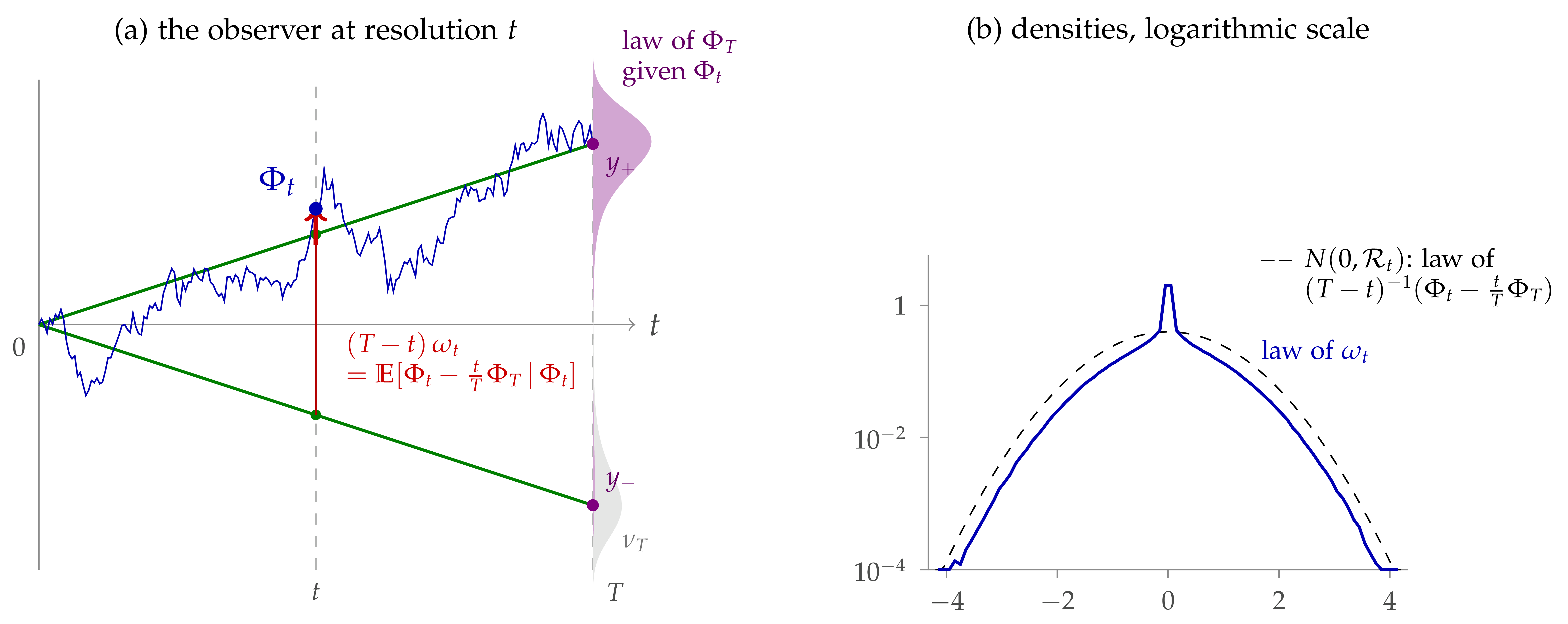
One mode: the Brownian bridge.

By (7.14) its position at time \(t\) is a point of the straight line from \(0\) to \(y\), plus a Gaussian deviation:

Then \(K \Phi_t - J_t F_t = \zeta_t / (T - t)\): with a known endpoint the noise is the rescaled deviation from the straight line, a centred Gaussian with variance \(t / (T (T - t)) = (T - t)^{- 1} - T^{- 1} =\mathcal{R}_t\), whatever \(y\). Now let the endpoint be random, with law \(\nu_T\). The observer at resolution \(t\) sees \(\Phi_t\), but not the line the path is following. The drift becomes the posterior mean of the bridge drift, and the noise the posterior mean of the rescaled deviation,

an average of Gaussian deviations, weighted by the posterior law of the endpoint (Figure 9.1, Exercise 9.6). Equivalently \(J_t F_t = K \Phi_t - \omega_t\), i.e. \(F_t = \Phi_t / t - (T / t) \omega_t\). The dictionary with the field is:

Figure 9.1. The noise as a posterior mean, for one mode with \(Q_t = t\), \(T = 1\), \(t = 1 / 2\), and the double-well terminal law \(\nu_T (\mathrm{d} y) \propto \mathrm{e}^{- 2 y^4 + 6 y^2} N (0, 1) (\mathrm{d} y)\) (grey, at time \(T\)). (a) A path observed up to time \(t\) (the faded part is not seen). For each possible endpoint \(y_{\pm}\) the bridge follows the straight line \(s \mapsto sy_{\pm} / T\) (green), and \(\Phi_t\) deviates from it by a Gaussian amount. The observer weighs the endpoints by their posterior law given \(\Phi_t\) (violet), and \((T - t) \omega_t\) is the posterior mean of the deviation (thick arrow). (b) The law of \(\omega_t\) (solid) has thinner tails than the Gaussian \(N (0, \mathcal{R}_t)\) of the deviation with a known endpoint (dashed): averaging thins the tails. The peak at \(0\) comes from the fields between the wells, where a small change of \(\Phi_t\) moves the posterior from one well to the other and \(\omega_t\) hardly changes, since the jump of the posterior mean compensates the motion of \(\Phi_t\): a fold of the map \(\Phi_t \mapsto \omega_t\) (Exercise 9.6(c)).

The general case.

and since \(J_t Q_t^{- 1} = K\),

The noise is minus the score of the law of the field at resolution \(t\), seen through \(J_t\).

Only deterministic covariance operators, all functions of \(A\), are commuted below. The variance that appears is the regulator (8.6) of the Wetterich equation: since \(S_t = Q_T (1 - J_t)\),

Proof. Write \(\Sigma_t = Q_t (1 - J_t)\), so that \(J_t \Sigma_t^{- 1} = S_t^{- 1}\), and \(g\) for the density of \(N (0, \Sigma_t)\). Then

and \(\mathrm{D} g (z) = - \Sigma_t^{- 1} z \hspace{0.17em} g (z)\), so

apply \(J_t\) and use (9.14). By conditional Jensen,

and \(S_t^{- 1} \zeta_t\) is centred Gaussian with covariance \(S_t^{- 1} \Sigma_t S_t^{- 1} =\mathcal{R}_t\).\(\Box\)

What the observer cannot resolve.

with \(\text{Cov}_t = \text{Cov} (\Phi_T |\mathcal{F}_t)\). The noise is the free bridge noise minus what the observer cannot resolve. The two extremes are the free field, where \(\text{Cov}_t = S_t\) and (9.17) gives \(KJ_t\), the covariance of \(KX_t\), and a strong pinning potential, where \(\text{Cov}_t \to 0\) and the bound is attained (Exercise 9.5). By Proposition 8.3, \(\text{Cov}_t = S_t - S_t \mathrm{D}^2 V_t (\Phi_t) S_t\), so that

the free value, corrected by the mean curvature of the effective potential. This is the analogue at resolution \(t\) of Nelson's covariance \(- \Delta + m^2 +\mathbb{E} [V'' (\varphi)]\), and here it is finite at every resolution. Proposition 9.6 is the same comparison for all convex functions, rather than for the variance alone.

For the heat profile (compare (8.15)), \(K = A \mathrm{e}^{A / T^2}\) and \(J_t = \mathrm{e}^{- A (t^{- 2} - T^{- 2})}\) give

(Exercise 9.5). At a finite spatial cutoff all of this holds with terminal resolution \(T = \infty\), before any continuum measure is constructed.

A new observation.

Tails of the force.

Proof. Two properties of \(V_t\) are used. (a) Semiconcavity. By Proposition 8.3, \(\mathrm{D}^2 V_t = S_t^{- 1} - S_t^{- 1} \text{Cov}_t S_t^{- 1} \leqslant S_t^{- 1}\) for every interaction, so

(b) Convexity. By (8.12), \(V_t\) is the infimal convolution of \(\Gamma_t\) with the convex quadratic \(\frac{1}{2} \langle \cdot, S_t^{- 1} \cdot \rangle\), hence convex. It is even, since \(V_T\) is and the Polchinski semigroup commutes with \(x \mapsto - x\).

Step 1. By (a) with \(a = uh\),

Integrate against \(\mu^{Q_t}\) and shift by the Cameron–Martin formula, \(\int G (x + a) \mu^{Q_t} (\mathrm{d} x) = \mathrm{e}^{- \frac{1}{2} \langle a, Q_t^{- 1} a \rangle} \int G (y) \mathrm{e}^{\langle Q_t^{- 1} a, y \rangle} \mu^{Q_t} (\mathrm{d} y)\):

Step 2. For every \(k\) the same shift gives \(\mathbb{E} \mathrm{e}^{\langle k, \Phi_t \rangle} = \mathrm{e}^{\frac{1}{2} \langle k, Q_t k \rangle} m (Q_t k) / m (0)\), with \(m (a) = \int \mathrm{e}^{- V_t (x + a)} \mu^{Q_t} (\mathrm{d} x)\). By (b) and Prékopa's theorem \(m\) is log-concave: it is the marginal of the log-concave function \((x, a) \mapsto \mathrm{e}^{- V_t (x + a) - \frac{1}{2} \langle x, Q_t^{- 1} x \rangle}\). It is also even, so \(\log m (0) \geqslant \frac{1}{2} \log m (a) + \frac{1}{2} \log m (- a) = \log m (a)\). Hence \(\mathbb{E} \mathrm{e}^{\langle k, \Phi_t \rangle} \leqslant \mathrm{e}^{\frac{1}{2} \langle k, Q_t k \rangle}\): the field at resolution \(t\) is no wider than the free field \(X_t\). With \(k = uQ_t^{- 1} h\) in (9.19) the two terms with \(Q_t^{- 1}\) cancel.\(\Box\)

Remark 9.8. (Where convexity enters) That convexity of \(\Gamma_t\) makes the force sub-Gaussian was remarked by Marcello Porta during the lectures. Step 1 uses only \(\mathrm{D}^2 V_t \leqslant S_t^{- 1}\), which holds for every interaction. Convexity of \(\Gamma_t\) enters only in Step 2, to compare \(\Phi_t\) with the free field. It is equivalent to \(\text{Cov}_t \leqslant S_t\) (Section 8.5): it holds at every \(t\) when \(V_T\) is convex, but for a double well, and for the Wick-ordered \(\Phi^4\) interaction, it can fail at low resolution, where the law of \(\Phi_t\) is wider than \(\mu^{Q_t}\). Without convexity, use the bridge (7.14) instead, \(\Phi_t = J_t \Phi_T + \zeta_t\) with \(\zeta_t \sim N (0, \Sigma_t)\) independent of \(\Phi_T\). Since \(J_t Q_t^{- 1} = K\) and \(Q_t^{- 1} \Sigma_t Q_t^{- 1} = Q_t^{- 1} - K\), (9.19) becomes

which also follows from \(F_t =\mathbb{E} [K \Phi_T - S_t^{- 1} \zeta_t | \Phi_t]\) (by (9.12) and Proposition 9.6) and conditional Jensen. The force is the noise plus the terminal field seen through \(K\): unlike the noise, it is sub-Gaussian uniformly in the interaction only when the terminal field is. For convex even \(V_T\), Step 2 at \(t = T\) bounds the last factor by \(\mathrm{e}^{\frac{u^2}{2} \langle h, Kh \rangle}\), and since \(\mathcal{R}_t + K = S_t^{- 1}\) this recovers (9.18). For one mode with \(V_T (y) = \kappa y^2 / 2\), \(F_t = - \kappa_t \Phi_t\) with \(\kappa_t = \kappa / (1 + \kappa S_t)\), and \(\text{Var} F_t = \kappa_t^2 / (Q_t^{- 1} + \kappa_t)\) increases to \(\mathcal{R}_t\) as \(\kappa \to \infty\): the bound \(S_t^{- 1} =\mathcal{R}_t + K\) is attained up to the term \(K\).

Convexity of the effective average action \(\Gamma^{\text{EAA}}_t = \Gamma_t + \frac{1}{2} \langle \cdot, K \cdot \rangle\) (Section 8.6) is not enough. Its gradient at the forecast is the noise, \(\mathrm{D} \Gamma^{\text{EAA}}_t (\psi_t) = K \psi_t - F_t = \omega_t\) by (9.12), which is sub-Gaussian with no assumption at all (Proposition 9.6); the force differs from it by \(K \psi_t\). Since \(\mathrm{D}^2 \Gamma^{\text{EAA}}_t = \text{Cov}_t^{- 1} -\mathcal{R}_t\) and \(\mathcal{R}_t = S_t^{- 1} J_t\), \(\Gamma^{\text{EAA}}_t\) is convex if and only if \(\text{Cov}_t \leqslant J_t^{- 1} S_t\), i.e. \(\mathrm{D}^2 V_t \geqslant - Q_t^{- 1}\): the law of \(\Phi_t\) is log-concave. This holds at \(t = 0\), where \(\Gamma^{\text{EAA}}_0\) is a Legendre transform, but a log-concave law may be much wider than \(\mu^{Q_t}\), and Step 2 needs \(\mathrm{D}^2 V_t \geqslant 0\). For one mode with \(Q_T = 1\), \(Q_t = q\) and the negative mass \(V_T (y) = - (1 - \varepsilon) y^2 / 2\), every \(\nu_t\) is Gaussian, so \(\Gamma^{\text{EAA}}_t\) is convex, but \(\text{Var} F_t = (1 - \varepsilon)^2 q / (\varepsilon (\varepsilon + q - q \varepsilon)) \sim 1 / \varepsilon\) while \(S_t^{- 1} = 1 / (1 - q)\).

The roughness of the noise.

Since \(x / (\mathrm{e}^x - 1) \leqslant \mathrm{e}^{- x / 2}\), \(\mathcal{R}_t \leqslant t^2 \mathrm{e}^{- A / 2 t^2}\): at resolution \(t\) the noise is no larger than \(t\) times a white noise smoothed at scale \(1 / t\). Pointwise, \(\operatorname{Var} \hspace{0.17em} \omega_t (x) \leqslant \mathcal{R}_t (x, x) \lesssim t^{d + 2}\), i.e. \(\omega_t (x) = O (t^{1 + d / 2})\). This is the size at scale \(1 / t\) of a distribution of regularity \(- 1 - d / 2\) (\(- 5 / 2\) in \(d = 3\)): seen at its own resolution, the noise is one derivative rougher than white noise (\(- d / 2\)) and two rougher than the GFF (\(1 - d / 2\)), the same as the GFF noise \(A \varphi = A^{1 / 2} \xi\) of the Dyson–Schwinger equation, whatever the interaction. It is not a bound on a limit distribution: \(\omega_t\) is a martingale in \(t\), not the smoothing of a fixed distribution, and on a fixed test function (9.16) only gives \(\langle h, \omega_t \rangle = O (t)\), while the free noise stays bounded. For \(\Phi^4_3\) no \(L^2\) limit of the logarithmic derivative is expected [ALZ06]. Compared with the free noise, the bound is sharp at and above the resolution, where \(\mathcal{R}_t / (A \mathrm{e}^{- A / t^2}) = (1 - \mathrm{e}^{- A / t^2})^{- 1} \to 1\), and larger by the factor \(t^2 / A\) on the resolved modes. Uniformly in the interaction it cannot be improved: for a pinning potential \(V_T = \frac{\kappa}{2} \| \varphi \|^2\), the covariance of \(\omega_t\) tends to \(\mathcal{R}_t\) as \(\kappa \to \infty\) (Exercise 9.5).

The noise as a stochastic observable.

This is the sense in which the Euclidean field equation of \(\Phi^4_3\) has a well-defined sub-Gaussian noise: it exists as a stochastic observable, without a terminal representative.

Remark 9.9. (Pathwise bounds) (sketch) Work at finite spatial cutoff, with \(T = \infty\) or \(t \leqslant T / 2\), so that \(\mathcal{R}_t\) obeys the bounds below uniformly in the cutoff. The norm

is convex, so Proposition 9.6 dominates \(\| \omega_t \|_{\varepsilon}\) by \(\| \Xi \|_{\varepsilon}\), with \(\Xi \sim N (0, \mathcal{R}_t)\). For this Gaussian field, \(\mathcal{R}_t (x, x) \lesssim t^{d + 2}\) and

so Dudley's bound and Gaussian concentration give Gaussian tails for \(\| \Xi \|_{\varepsilon}\) at the level \(t^{1 + d / 2} \sqrt{\log (2 + t)}\), uniformly in \(L\). Since \(\omega\) is a martingale, \(\| \omega_s \|_{\varepsilon}\) is a submartingale, and Doob's inequality extends the tails to \(\sup_{s \leqslant t}\). Summing over dyadic \(t\), almost surely, with a random constant \(\tilde{C}\),

with \(\tilde{C}\) having Gaussian tails uniformly in the interaction and in the spatial cutoff. This is a pathwise bound at each resolution, in the sense above.

Control of the force.

so

Itô's isometry, \((a + b)^2 \leqslant 2 a^2 + 2 b^2\) and (9.16) give

For the heat profile with \(T = \infty\), \(KQ_t K = A \mathrm{e}^{- A / t^2} \leqslant t^2 / \mathrm{e}\), so the right-hand side is at most \(2 (1 + \mathrm{e}^{- 1}) t^2 \|h\|_{L^2}^2\). This controls a smoothed derivative of the force, \(\Upsilon_s = \mathrm{D} F_s (\Phi_s) \dot{Q}_s^{1 / 2}\), without any estimate on the terminal force.

Consequence for \(\Phi^4_3\).

9.5Infinite volume

On \(\mathbb{T}^d_L\) the free energy \(V_0 (0)\) and the effective potential \(V_t\) are extensive: they grow like \(L^d\), and (7.9) has no limit as \(L \to \infty\). Three objects are intensive and survive formally:

Differences of free energies.

Proof. By (7.12), the left-hand side is \(\inf_u J_f (u) - J_0 (u^{\ast})\), with

Writing \(u = u^{\ast} + w\) and expanding \(\frac{1}{2} \|u^{\ast} + w\|^2\), the terms \(V_T (\Phi_T)\) and \(\frac{1}{2} \int \|u^{\ast} \|^2\) cancel against \(J_0 (u^{\ast})\), and the cross term is computed above. The first-order condition in \(w\) is obtained as in (7.11).\(\Box\)

For a local interaction \(V_T (\varphi) = \int v_T (\varphi (x)) \mathrm{d} x\),

and \(b_T (a, 0) = 0\). So every term of (9.22) is local: there is no free energy and no extensive quantity, only the field \(\Phi\) and the perturbation that \(f\) induces on it. For \(f\) supported in a bounded region one expects the optimal \(w\), and with it \(I (w)\), to decay away from the support, at the rate of the decay of correlations of the measure. Both sides of (9.22) then make sense in infinite volume, with \(\Phi\) a solution of the infinite-volume FBSDE (9.21). This suggests the following formal description of the infinite-volume measures (at a fixed ultraviolet cutoff \(T\)):

The Laplace functionals in (9.22) determine the measure, and the condition involves only intensive quantities. When the FBSDE has several solutions, as is expected in the presence of phase transitions, each solution gives a measure with its own variational principle; the perturbations \(w\) of finite energy only probe a given solution locally. For \(\Phi^4_3\) this remainder term contains the divergent counterterms, and, as for (7.12), the change of variables of [BG20] is needed before (9.22) has bounds uniform in \(T\); in two dimensions, compare the infinite-volume analysis of [BG23].

The coercive estimates must then be local: one uses weighted norms and needs bounds whose constants do not depend on the volume. This infrared problem is the analogue, for the scale dynamics, of the “coming down from infinity” estimates for the parabolic dynamics.

Exercises

Appendices: additional material

Appendix AAlgebraic structure of the Polchinski flow

A.1A semigroup of renormalisation maps

For a positive covariance \(S\) define the renormalisation map

Since \(\mu^S \ast \mu^{S'} = \mu^{S + S'}\),

So the effective potentials are an orbit of an abelian semigroup, indexed by the cone of positive covariances, acting nonlinearly on interactions and linearly on Boltzmann factors \(\mathrm{e}^{- V}\). Its infinitesimal generators are the vector fields

and (7.8) reads \(\partial_t V_t = -\mathcal{P}_{\dot{Q}_t} (V_t)\).

Proof. (a) Differentiate \(\mathfrak{R}_{sB} \mathfrak{R}_{rB'} =\mathfrak{R}_{rB'} \mathfrak{R}_{sB}\) at \(s = r = 0\), or compute directly (Exercise A.1). (b) is (A.2).\(\Box\)

Different profiles with the same endpoints are different coordinate systems on the same renormalisation group trajectory. They change the process \(\Phi\) and the observables at intermediate resolution, but not the terminal theory. The flow has no holonomy [BCG26].

A.2Perturbation theory and counterterms

Expanding \(V_t =\mathfrak{R}_{Q_{T, t}} (V_T)\) in cumulants of the Gaussian increment \(\zeta \sim \mu^{Q_{T, t}}\) gives

For (7.1), Exercise 6.1 of Lecture 3 shows that Gaussian convolution simply lowers the Wick ordering: since \(Q_{T, t} (x, x) = c_T - c_t\),

Here \(\gamma_T = O (\lambda^2)\) is kept for later use. At first order the effective potential is the Wick-ordered potential at the current resolution. This is the dual statement of Proposition 6.1 of Lecture 3: \(\int H_4 (X_t ; c_t)\) is an observable.

Proof. By the binomial formula for Hermite polynomials,

Then compute the variance in (A.4) with Lemma 3.8 of Lecture 2.\(\Box\)

Figure A.1. The terms \(k = 1, 2, 3, 4\) of (A.6), with \(k\) lines \(S\) joining two Wick-ordered vertices; Wick ordering has removed the lines from a vertex to itself. As \(T \to \infty\) in \(d = 3\), only the sunset, \(k = 3\), is a non-integrable divergence for the \(: \varphi^2 :\) term; it is cancelled by \(\gamma_T\).

Now let \(T \to \infty\) at fixed \(t\), so that \(S \to C - Q_t\), which near the diagonal is as singular as \(G\). In \(d = 2\) every \(S^k\) is locally integrable, so with \(\gamma_T = 0\) every term has a limit: Wick ordering suffices. In \(d = 3\), \(G (z) \sim (4 \pi |z|)^{- 1}\):

• \(k = 1, 2\): \(S\) and \(S^2\) are locally integrable. These terms are finite and nonlocal.

• \(k = 3\) (the sunset): \(S^3 \sim |z|^{- 3}\) is not integrable. Writing \(\phi (x) \phi (y) = \frac{1}{2} (\phi (x)^2 + \phi (y)^2) - \frac{1}{2} (\phi (x) - \phi (y))^2\), up to a field-independent constant the divergent part is local:

  \(\displaystyle - \frac{\lambda^2}{3} \left( \int S^3 \right) \int : \phi^2 :_t + \text{ (finite)},\)

  with \(\int S^3 \sim \frac{1}{16 \pi^2} \log T\). It is cancelled by

  \(\displaystyle \gamma_T := \frac{\lambda^2}{3} \int_{\mathbb{T}^3_L} Q_T (z)^3 \hspace{0.17em} \mathrm{d} z = \frac{\lambda^2}{48 \pi^2} \log T + O (1),\)

  (A.7)

  since \(\gamma_T - \frac{\lambda^2}{3} \int S^3\) converges (Exercise A.2).

• \(k = 4\): a divergent constant \(- \frac{\lambda^2}{12} L^3 \int S^4 \sim T\), the vacuum energy. It cancels in \(\nu_T\) but not in the free energy.

Power counting (Exercise A.3) shows that no further field-dependent counterterms are needed in \(d = 3\): \(\Phi^4_3\) is superrenormalisable. Thus renormalisation appears as a property of the flow: one chooses the terminal data \(V_T\) so that the effective potentials \(V_t\) at fixed resolution have limits. The divergences at second order are also related to the singularity of \(\Phi^4_3\) with respect to the GFF [BG21]: the measures \(\nu_t\) at fixed \(t\) are expected to stay absolutely continuous with respect to \(\mu^{Q_t}\), while the terminal one is not.

Exercises

Appendix BStochastic localisation

Proposition 7.2 and Section 7.3 say that the Polchinski process is a stochastic localisation of \(\nu_T\). This appendix records why that decomposition is useful, and what it proves.

Why it is useful.

• It is a martingale. \(\nu_T =\mathbb{E} \mu_t^{\Phi_t}\), and the expectation of any test function under \(\mu_t^{\Phi_t}\) is a martingale. Itô calculus then splits variance and entropy exactly into the part already revealed and the part still hidden.

• The pieces are simpler. The Gaussian factor adds \(\mathcal{R}_t\) to the Hessian of the potential. If \(\nu_T\) is log-concave, \(\mu_t^{\phi}\) is \(\mathcal{R}_t\)-uniformly log-concave, so Bakry–Émery and Brascamp–Lieb apply to it even when their constants are useless for \(\nu_T\) itself.

• One quantity controls the loss. What is revealed per unit resolution is governed by \(\operatorname{Cov}_t\), whose evolution (8.9) is explicit. An inequality for \(\nu_T\) reduces to showing that the localisation does not happen too fast.

The process can also be run as an algorithm: with an approximate force it is a sampler, as in the algorithmic stochastic localisation of [EMS22], and denoising diffusions are of the same kind [Mon23]. By (9.14), the noise of the field equation is, up to \(J_t\), the score that such algorithms estimate.

B.1Log-Sobolev inequalities along the localisation

Bauerschmidt and Bodineau [BB21] proved log-Sobolev inequalities by running the Polchinski flow (see the survey [BBD24]). In their language the renormalised measure at a given scale is the law of \(\Phi_t\), and the fluctuation measure is the conditional law \(\mu_t^{\Phi_t}\) of Proposition 7.2, i.e. the stochastic localisation of \(\nu_T\) [Eld23]. (Their scale parameter runs opposite to our resolution: their initial scale is our \(T\), where the renormalised measure is \(\nu_T\) and the fluctuation measure is trivial, and their integrated covariance is our \(S_t\).) In this dictionary their argument is an entropy computation along our filtration.

Entropy as quadratic variation.

and, stopping at resolution \(t\), the chain rule

the entropy already revealed at resolution \(t\) plus the expected entropy still hidden. The increments are controlled by the conditional law: differentiating the density of \(\mu_t^{\phi}\) in \(\phi\), \(\mathrm{D} G_t (\phi) = S_t^{- 1} \operatorname{Cov}_{\mu_t^{\phi}} (\rho, y)\).

The hypothesis gives, at each resolution, the gradient bound

inserted in the entropy formula it gives the theorem [BBD24]. For \(V_T = 0\) and a linear profile \(Q_t = tQ_T / T\) one may take \(\kappa = 0\), so \(1 / \varrho = T\) and the theorem is the Gaussian log-Sobolev inequality \(\operatorname{Ent} (\rho) \leqslant 2\mathbb{E} \langle D \sqrt{\rho}, Q_T D \sqrt{\rho} \rangle\). The hypothesis is a convexity condition on the effective potentials at every scale, not on \(V_T\), corrected by the scale dependence \(\ddot{Q}_t\) of the decomposition; \(\kappa_t\) may be negative at some scales: only the weights \(\mathrm{e}^{- 2 \int_t^T \kappa_r \mathrm{d} r}\) enter \(\varrho\).

In terms of the conditional covariance.

If \(\dot{Q}_t\) is invertible, multiplying on the left by \(S_t \dot{Q}_t^{- 1} = \dot{\mathcal{R}}_t^{- 1} S_t^{- 1}\) and on the right by its transpose \(\dot{Q}_t^{- 1} S_t\) shows that it is equivalent to the explicit bound

The second derivative \(\ddot{Q}_t\) is not estimated: it is a property of the Gaussian decomposition, and it enters only through the combination \(\kappa_t \dot{Q}_t - \frac{1}{2} \ddot{Q}_t\). When \(Q_t\) and \(S_t\) are functions of one operator (Fourier multipliers, say), the right-hand side is \(S_t - S_t^2 \dot{Q}_t^{- 2} (\kappa_t \dot{Q}_t - \frac{1}{2} \ddot{Q}_t)\) mode by mode. If \(\kappa_t \dot{Q}_t > \frac{1}{2} \ddot{Q}_t\) (for the linear profile: \(\kappa_t > 0\)), every conditional law is strictly more concentrated than the unresolved Gaussian fluctuation; if not, \(\operatorname{Cov}_t\) may exceed \(S_t\), as in a double well at low resolution. A concave profile (\(\ddot{Q} \leqslant 0\)) makes the bound smaller but forces \(\kappa\) down by the same amount: for the Gaussian with \(Q_t = 1 - \mathrm{e}^{- t}\) one has \(\ddot{Q} = - \dot{Q}\), the hypothesis holds with \(\kappa = - \frac{1}{2}\), and \(\operatorname{Cov}_t = S_t\). The hypothesis is thus an upper bound on the conditional covariance, uniform in the conditioning, measured in the metric \(\dot{\mathcal{R}}_t\). Closely related is the entropic stability of Chen and Eldan [CE22] (see also [BBD24]): if, for all \(r \leqslant t\) and all \(\phi\), \(\dot{\mathcal{R}}_r \operatorname{Cov}_{\mu_r^{\phi}} \dot{\mathcal{R}}_r \leqslant \alpha_r \dot{\mathcal{R}}_r\), then

the total entropy is controlled by the entropy that is still hidden at resolution \(t\). The low-resolution part of the localisation is where the measure may be multimodal, and the condition says that it does not hide too much. With the Brascamp–Lieb bounds of Section 8.4 the conditional covariance is controlled by the Hessian of \(V_T\) when this is convex; for \(\Phi^4_3\) it is not, and the condition is a statement about the effective potentials, i.e. about the renormalisation group flow itself.

Proof. Let \(M_r =\mathbb{E}_r f (\Phi_T)\) and \(\chi_r =\operatorname{Cov}_{\mu_r^{\Phi_r}} (f, y)\). As in Section B.1, \(\mathrm{d} \langle M \rangle_r = \langle \chi_r, \dot{\mathcal{R}}_r \chi_r \rangle \mathrm{d} r\), so \(v (r) := \mathbb{E}\operatorname{Var}_{\mu_r^{\Phi_r}} (f)\) has \(v' = -\mathbb{E} \langle \chi_r, \dot{\mathcal{R}}_r \chi_r \rangle\) and \(v (0) =\operatorname{Var}_{\nu_T} (f)\). By Cauchy–Schwarz, with \(h = \dot{\mathcal{R}}_r \chi_r\), \(\langle \chi_r, h \rangle^2 \leqslant \operatorname{Var}_{\mu_r^{\Phi_r}} (f) \langle h, \operatorname{Cov}_r h \rangle \leqslant \alpha_r \operatorname{Var}_{\mu_r^{\Phi_r}} (f) \langle \chi_r, \dot{\mathcal{R}}_r \chi_r \rangle\). Hence \(v' \geqslant - \alpha_r v\), which gives the first bound. For the second, the Hessian of the potential of \(\mu_t^{\phi}\) is at least \(\mathcal{R}_t\): apply Brascamp–Lieb to \(\mu_t^{\phi}\) and take the expectation.\(\Box\)

For \(V_T = 0\) one has \(\operatorname{Cov}_r = S_r\). In one mode, or for the linear profile, where \(\dot{Q}_r S_r^{- 1}\) is a number, \(\alpha_r = \dot{Q}_r S_r^{- 1}\) and \(\exp \int_0^t \alpha_r \mathrm{d} r = Q_T S_t^{- 1}\): the first bound is an equality for linear \(f\), and the second tends to the Gaussian Poincaré inequality as \(t \to T\) (Exercise B.2).

An application: the KLS conjecture.

The connection with Bauerschmidt–Bodineau.

Proposition 8.3 is the bridge: convexity of the renormalised potentials is an upper bound on the conditional covariance, namely (B.1). The two methods then use this information differently.

• Bauerschmidt–Bodineau. The Kolmogorov equation (9.2) transports \(G_t\) by the drift \(\dot{Q}_t F_t = - \dot{Q}_t \mathrm{D} V_t\). Its Jacobian plays the role of the curvature in the Bakry–Émery computation, and the scale dependence of the metric \(\dot{Q}_t\) adds \(\frac{1}{2} \ddot{Q}_t\). This yields the gradient bound for \(G_t\) at each scale, which is integrated in the entropy formula. The output is a log-Sobolev inequality with an explicit constant, directly at the terminal scale, also far from log-concavity. The hypothesis is uniform in \(\phi\), which suits field theories where the renormalisation group controls \(V_t\) for all fields, as for sine-Gordon at \(\beta < 6 \pi\) [BB21].

• Localisation. One bounds what is lost on \([0, t]\) (the proposition above, or entropic stability [CE22]) and uses a known inequality for \(\mu_t^{\phi}\). It works directly with moments of the conditional law, and can use bounds that hold only with high probability along the path, as in the KLS problem.

Exercises

References

[ALZ06]

S. Albeverio, S. Liang, B. Zegarlinski. Remark on the integration by parts formula for the \(\varphi^4_3\)-quantum field model. Infin. Dimens. Anal. Quantum Probab. Relat. Top. 9 (2006), 149–154.

[AY02]

S. Albeverio, M. W. Yoshida. \(H\)-\(C^1\) maps and elliptic SPDEs with polynomial and exponential perturbations of Nelson's Euclidean free field. J. Funct. Anal. 196 (2002), 265–322.

[BB19]

R. Bauerschmidt, T. Bodineau. A very simple proof of the LSI for high temperature spin systems. J. Funct. Anal. 276 (2019), 2582–2588.

[BB21]

R. Bauerschmidt, T. Bodineau. Log-Sobolev inequality for the continuum sine-Gordon model. Comm. Pure Appl. Math. 74 (2021), 2064–2113.

[BBD24]

R. Bauerschmidt, T. Bodineau, B. Dagallier. Stochastic dynamics and the Polchinski equation: an introduction. Probab. Surveys 21 (2024), 200–290.

[BCG26]

I. Bailleul, I. Chevyrev, M. Gubinelli. Stochastic observables and Wilson–Itô diffusions. In preparation.

[BG20]

N. Barashkov, M. Gubinelli. A variational method for \(\Phi^4_3\). Duke Math. J. 169 (2020), 3339–3415.

[BG21]

N. Barashkov, M. Gubinelli. The \(\Phi^4_3\) measure via Girsanov's theorem. Electron. J. Probab. 26 (2021), 1–29.

[BG23]

N. Barashkov, M. Gubinelli. On the variational method for Euclidean quantum fields in infinite volume. Probab. Math. Phys. 4 (2023), 761–801.

[CE22]

Y. Chen, R. Eldan. Localization schemes: a framework for proving mixing bounds for Markov chains. In 2022 IEEE 63rd Annual Symposium on Foundations of Computer Science (FOCS), 2022, 110–122.

[Che21]

Y. Chen. An almost constant lower bound of the isoperimetric coefficient in the KLS conjecture. Geom. Funct. Anal. 31 (2021), 34–61.

[Eld13]

R. Eldan. Thin shell implies spectral gap up to polylog via a stochastic localization scheme. Geom. Funct. Anal. 23 (2013), 532–569.

[Eld23]

R. Eldan. Analysis of high-dimensional distributions using pathwise methods. In Proceedings of the ICM 2022, EMS Press, 2023, 4246–4270.

[EMS22]

A. El Alaoui, A. Montanari, M. Sellke. Sampling from the Sherrington–Kirkpatrick Gibbs measure via algorithmic stochastic localization. In 2022 IEEE 63rd Annual Symposium on Foundations of Computer Science (FOCS), 2022.

[GH21]

M. Gubinelli, M. Hofmanová. A PDE construction of the Euclidean \(\Phi^4_3\) quantum field theory. Comm. Math. Phys. 384 (2021), 1–75.

[GJS75]

J. Glimm, A. Jaffe, T. Spencer. Phase transitions for \(\varphi^4_2\) quantum fields. Comm. Math. Phys. 45 (1975), 203–216.

[KL22]

B. Klartag, J. Lehec. Bourgain's slicing problem and KLS isoperimetry up to polylog. Geom. Funct. Anal. 32 (2022), 1134–1159.

[KL24]

B. Klartag, J. Lehec. Affirmative resolution of Bourgain's slicing problem using Guan's bound. Preprint, arXiv:2412.15044, 2024.

[Kla23]

B. Klartag. Logarithmic bounds for isoperimetry and slices of convex sets. Ars Inven. Anal. (2023), Paper No. 4.

[Mon23]

A. Montanari. Sampling, diffusions, and stochastic localization. Preprint, arXiv:2305.10690, 2023.

[Nel75]

E. Nelson. Remarks on Markov field equations. In A. M. Arthurs (ed.), Functional Integration and its Applications, Clarendon Press, Oxford, 1975, 136–143.